050 — The Vreeswijk-Sompolinsky asynchronous-irregular state
Abstract
Cortical neurons fire irregularly — their spike trains look almost like random (Poisson) processes, even though a single neuron driven by steady current fires like clockwork. Vreeswijk & Sompolinsky’s 1996 Science paper explained why: in a recurrent network where excitation and inhibition are both strong and roughly cancel, what’s left over is fluctuations, and cells fire when those fluctuations randomly push them over threshold. The result is the asynchronous-irregular (AI) state — moderate rates, near-Poisson spiking, low correlations between cells, and deterministic chaos. This entry reproduces that state on the same conductance-based network used elsewhere in this collection to produce gamma-rhythmic PING, and checks all four of V&S’s signatures against a PING control. The same architecture gives two completely different regimes depending only on how it’s wired and driven.
The idea
A leaky integrate-and-fire neuron given a constant supra-threshold current is a metronome: it charges to threshold, fires, resets, repeats — perfectly regular, CV (coefficient of variation of inter-spike intervals) = 0. Real cortical neurons have CV ≈ 1, the value you’d get from a Poisson process. Where does the randomness come from?
V&S’s answer: not from noisy inputs, but from the balance of strong recurrent excitation and inhibition. Picture a cell receiving excitatory and inhibitory recurrent inputs, each of strength . The mean excitatory and inhibitory currents are each large () but opposite-signed, so they cancel — the cell sits near threshold, not far above it. What survives the cancellation is the fluctuation around the mean (also by the central limit theorem). With the mean drive parked near threshold and fluctuations of comparable size, every spike is triggered by a chance upward swing. Firing becomes a threshold-crossing of noise, which is approximately Poisson.
This is self-organising: the network finds the firing rates at which the E and I currents balance, no fine-tuning required. It’s robust, it’s generic, and it produces four hallmarks that can each be measured:
- Irregular — single-cell ISI distributions approach Poisson, CV → 1.
- Asynchronous — pairs of cells are nearly uncorrelated (correlation , vanishing for large ).
- Fluctuation-driven — the fluctuation amplitude is comparable to or larger than the distance from mean drive to threshold.
- Chaotic — a tiny perturbation to the network state grows (positive Lyapunov exponent); the network never settles onto a periodic orbit.
Brunel (2000) showed the regime survives the move from V&S’s binary-spin neurons to spiking LIF neurons; Renart et al. (2010) showed it survives conductance-based synapses. So we should be able to reach it on our conductance-based LIF network too — and contrast it against the gamma-clocked PING state the same network produces in other operating points.
Building it
We run two cells of the same network (COBANet, , , ms, ms): a PING control (the gamma-rhythmic regime, our foil) and a V&S AI target. They differ only in connectivity and drive:
| PING (control) | V&S AI | |
|---|---|---|
| Recurrent connectivity | dense | fixed fan-in: exactly inputs per cell |
| coupling () | none | μS |
| / | biophysical PING defaults | / μS |
| External drive | 20 Hz Poisson through | per-cell independent Poisson on E (45 Hz) and I (8 Hz), bypassing |
Three ingredients are what the PING runs never use, each mapping directly onto a V&S assumption:
- An matrix. PING has no inhibitory self-coupling; V&S needs it so the inhibitory population doesn’t fire in synchronous bursts (which would re-establish a rhythm).
- Fixed- connectivity. Every cell draws exactly presynaptic inputs (V&S’s assumption that all cells are statistically equivalent). The obvious alternative — zeroing each weight independently with probability — gives a binomial fan-in that varies cell to cell (mean 10, but range 2–21), which broadens the rate distribution. Switching to fixed- cut the spread of per-cell rates from CV to .
- Per-cell independent drive on both populations. Each cell gets its own private Poisson noise stream into its excitatory conductance. This is the uncorrelated external input V&S’s cells receive. (Driving only E and letting I inherit noise through leaves the I cells too correlated; both populations need their own.)
The headline result, before the diagnostics:
| PING | V&S AI | |
|---|---|---|
| 4, 31 Hz | 17, 21 Hz | |
| Raster | gamma bands | scattered |
| Welch PSD | sharp 31 Hz peak | broadband, no peak |
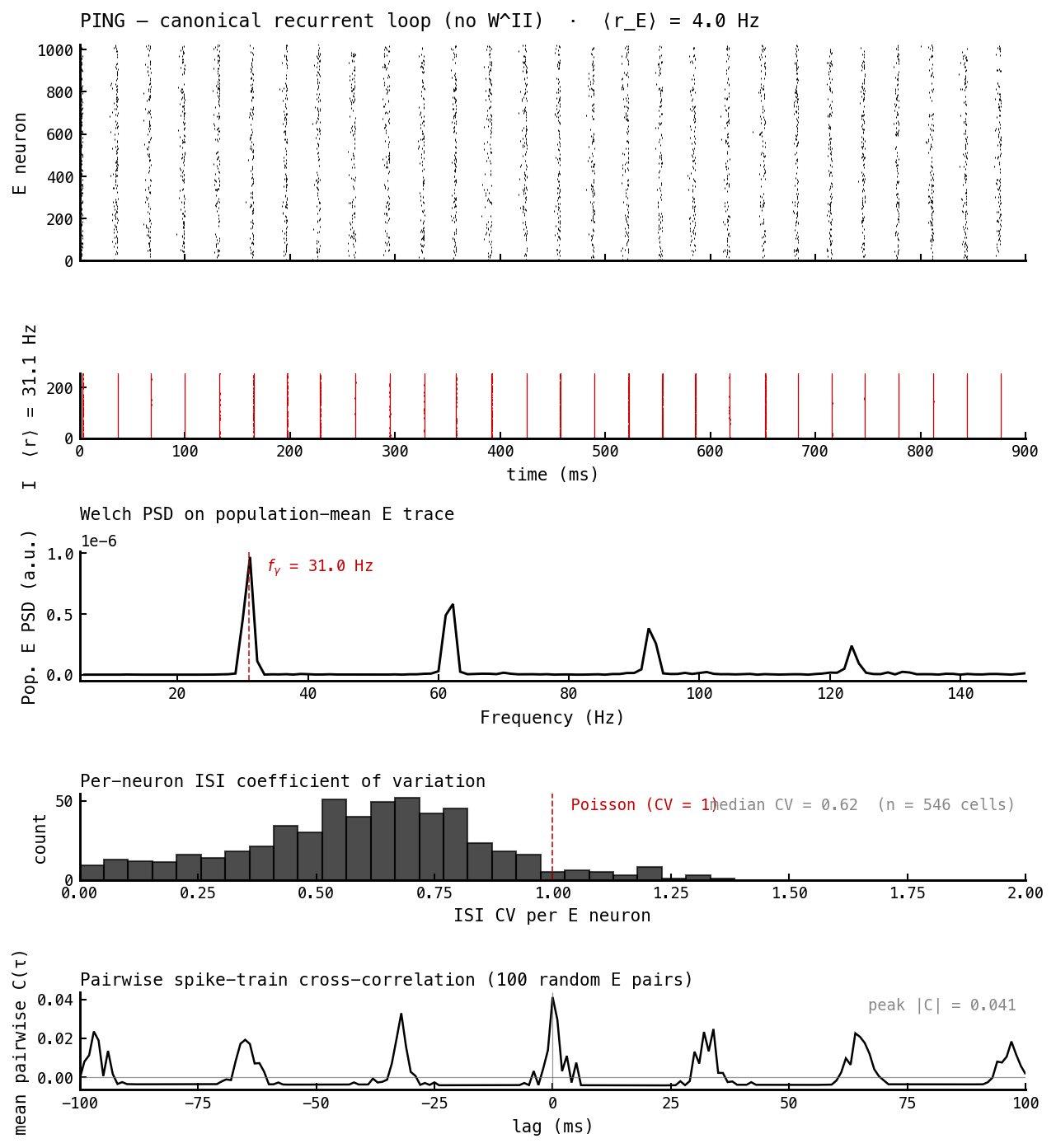
The foil. PING fires in cycle-locked gamma bursts: a sharp spectral peak, regular (sub-Poisson) ISIs, and cross-correlations that comb at the gamma period. Everything the AI state is not.
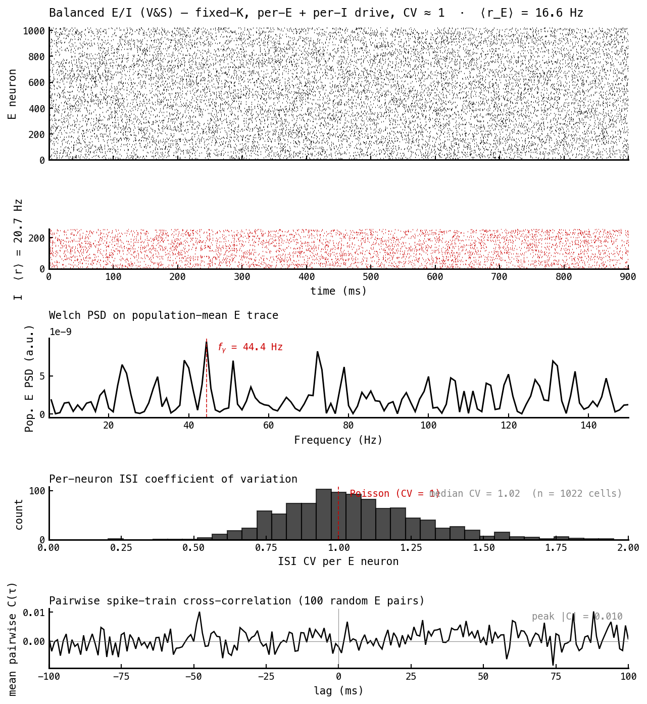
The target. Scattered rasters, broadband spectrum, ISIs centered on Poisson, flat cross-correlations. The same five panels as Figure 1, telling the opposite story.
Checking the four signatures
Each row of the contrast below is one V&S prediction, confirmed against the PING foil.
| Signature | PING | V&S AI | V&S predicts |
|---|---|---|---|
| Irregular — median ISI CV | 0.62 / 0.03 (E/I) | 1.02 / 1.13 | → 1 |
| Asynchronous — peak |pairwise C(τ)| | 0.041 (gamma comb) | 0.010 (flat) | → 0 |
| Fluctuation-driven — median | 5.5 | 23 | |
| Chaotic — divergence after ε kick | re-locks to 0 | sustained ≈ 6 cells | grows () |
1 & 2: Irregular and asynchronous
These two read directly off Figures 1 and 2. Irregularity is the ISI-CV histogram (panel 4): PING’s E cells are regular (CV 0.62) and its I cells almost perfectly periodic (0.03, a metronome), while the AI cell’s E and I CVs both sit at ≈ 1 — Poisson. Asynchrony is the cross-correlogram (panel 5): PING shows a comb of peaks at multiples of the gamma period (cells that fire together this cycle fire together next cycle), whereas the AI correlogram is flat noise with a 4× smaller peak — cells fire essentially independently.
3: Fluctuation-driven firing
The mechanistic core of the theory: cells fire because fluctuations push them over threshold, not because the mean drive is supra-threshold. We measure this per cell from the total membrane current : its time-mean , its time-std , and the ratio
where nA is the current that just holds a cell at threshold. means fluctuations dwarf the gap to threshold — fluctuation-driven firing.
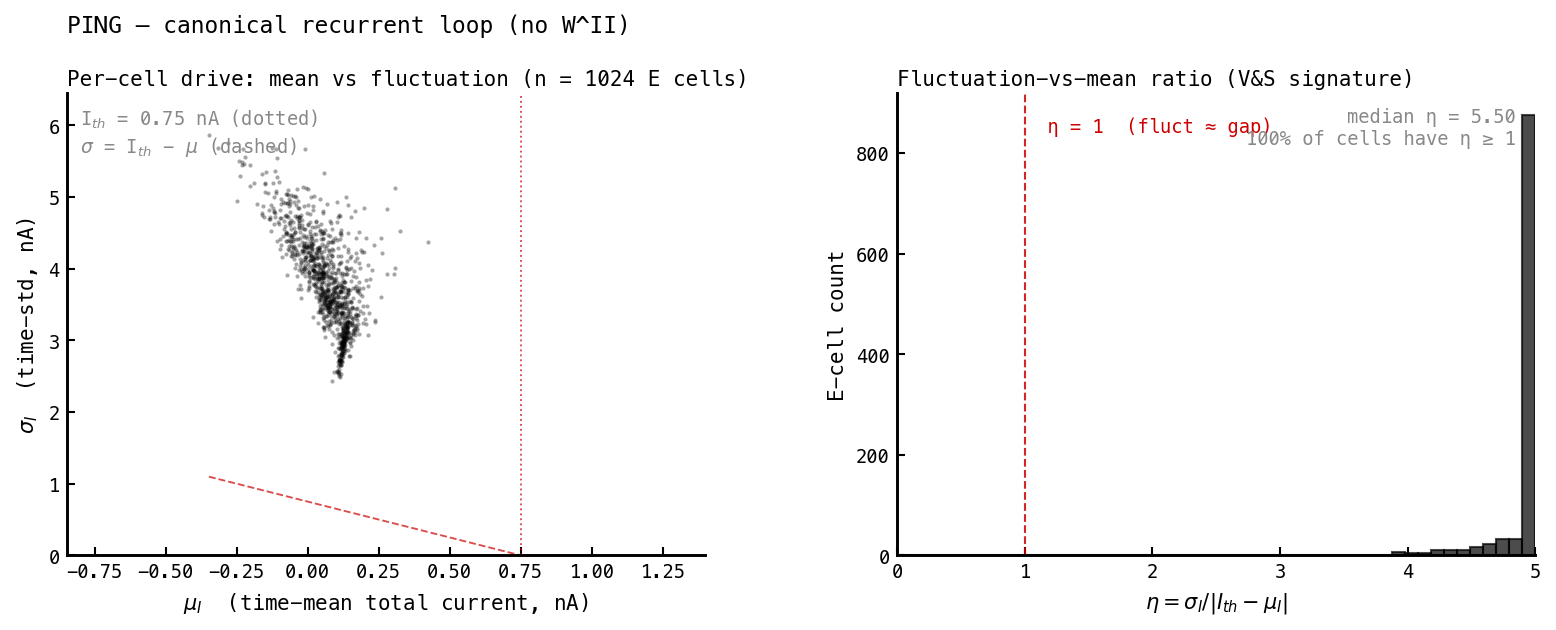
PING. Mean drives cancel to (well below threshold), but is large — the fluctuations here are the deterministic gamma-cycle pumps, not random noise. So PING technically satisfies too, but its fluctuations are a clock, which the spectrum and correlogram already exposed.
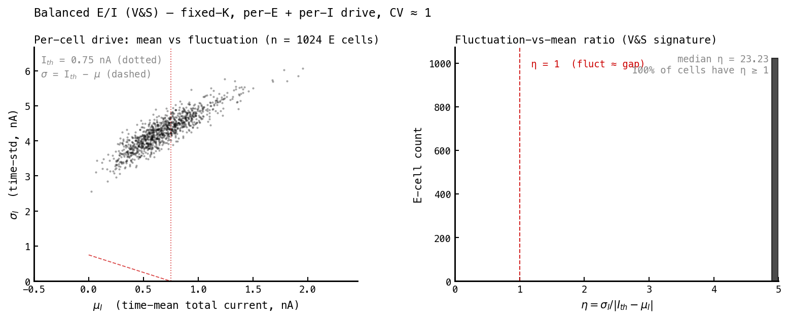
V&S AI. Mean drive sits right at threshold () with fluctuations many times larger ( nA). Median — every cell is strongly fluctuation-dominated, and here the fluctuations are genuinely random (independent Poisson noise), which is what makes the firing Poisson.
4: Chaos
The sharpest test of all, and the one that separates “balanced and noisy” from “balanced and chaotic.” Clone the network, perturb every membrane voltage by a tiny ε = 2 mV at , and rerun on identical frozen input (same Poisson stream, same seed). Track = the number of E cells whose spike differs between the two copies. A chaotic network amplifies the perturbation; a stable one forgets it.
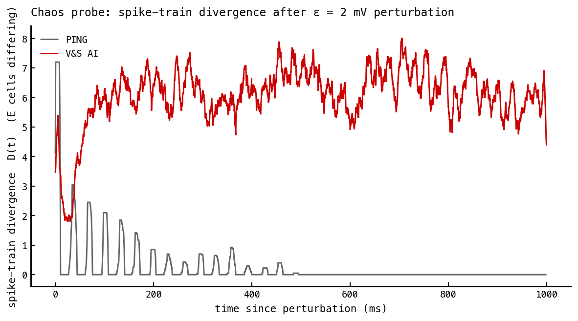
PING forgets the kick; AI does not. PING (grey) re-locks: the perturbation rings down in decaying gamma-period pulses and reaches exactly zero — a stable limit cycle (). The AI cell (red) saturates at a sustained ≈ 6-cell divergence and never returns to zero — the perturbation grows then plateaus, the signature of positive (chaos).
The divergence saturates at a modest level (a handful of cells out of 1024) because the strong shared input partly entrains both copies — strongly-driven neurons fire reliably regardless of network state (the Mainen-Sejnowski effect). So our cell is “noise-entrained with chaos on top” rather than V&S’s strongly-autonomous chaos. But the qualitative split is unambiguous: PING’s perturbation vanishes to exactly zero, AI’s persists.
How faithful is it?
All four V&S signatures reproduce on a conductance-based LIF network — irregular, asynchronous, fluctuation-driven, chaotic — side-by-side with a PING control that fails every one. Two honest caveats remain:
- Hand-tuned, not derived weights. V&S derive the synaptic scaling from the requirement that fluctuations stay as . We found our operating point by tuning on the diagnostics rather than imposing that scaling. The state is clearly in the right regime, but we haven’t verified the mean E and I currents are individually -large and cancelling.
- Weak chaos, masked by input entrainment. Because our cells are driven by strong shared Poisson noise, the perturbation can’t grow far before the common input re-entrains both copies. The autonomous chaos of V&S’s quenched-input network would show much larger divergence.
Both are sharpenings, not contradictions — the regime is V&S; the remaining work is making it quantitatively V&S.
Next steps
- scaling check. Sweep at fixed with weights rescaled and confirm the state is -invariant (CV, rate, spectrum unchanged). This is what would prove we’re on the V&S balanced manifold rather than at a lucky single- operating point. Fixed- connectivity, added here, is the prerequisite.
- Quenched-input chaos. Replace the fresh per-timestep Poisson drive with a frozen DC offset per cell, so the Lyapunov probe measures autonomous network chaos without the input-entrainment mask.