June 15th lab meeting presentation
E neurons (driven by feedforward input and inhibitory feedback):
I neurons (driven by excitatory feedback only; no inhibitory input):
- — membrane potential of E and I populations at step (mV)
- — excitatory / inhibitory conductances on E neurons (µS)
- — excitatory conductance on I neurons (µS); I receives no inhibition
- — per-step aggregate conductance, effective membrane time constant, steady-state voltage
- — membrane capacitance (1.0 nF on E, 0.5 nF on I)
- — leak conductance (0.05 µS on E, 0.1 µS on I) and reversal potential (−65 mV)
- — synaptic reversal potentials (0 mV, −80 mV)
- — spike threshold (−50 mV) and reset voltage (−65 mV)
- — refractory periods (3 ms, 1.5 ms)
- — per-step AMPA decay factor ( ms)
- — per-step GABA decay factor ( ms)
- — feedforward (trained), E→I, and I→E weight matrices ( µS, µS at PING init )
- — input, excitatory, and inhibitory spike trains at step
- — integration timestep (0.1 ms)
Architectures
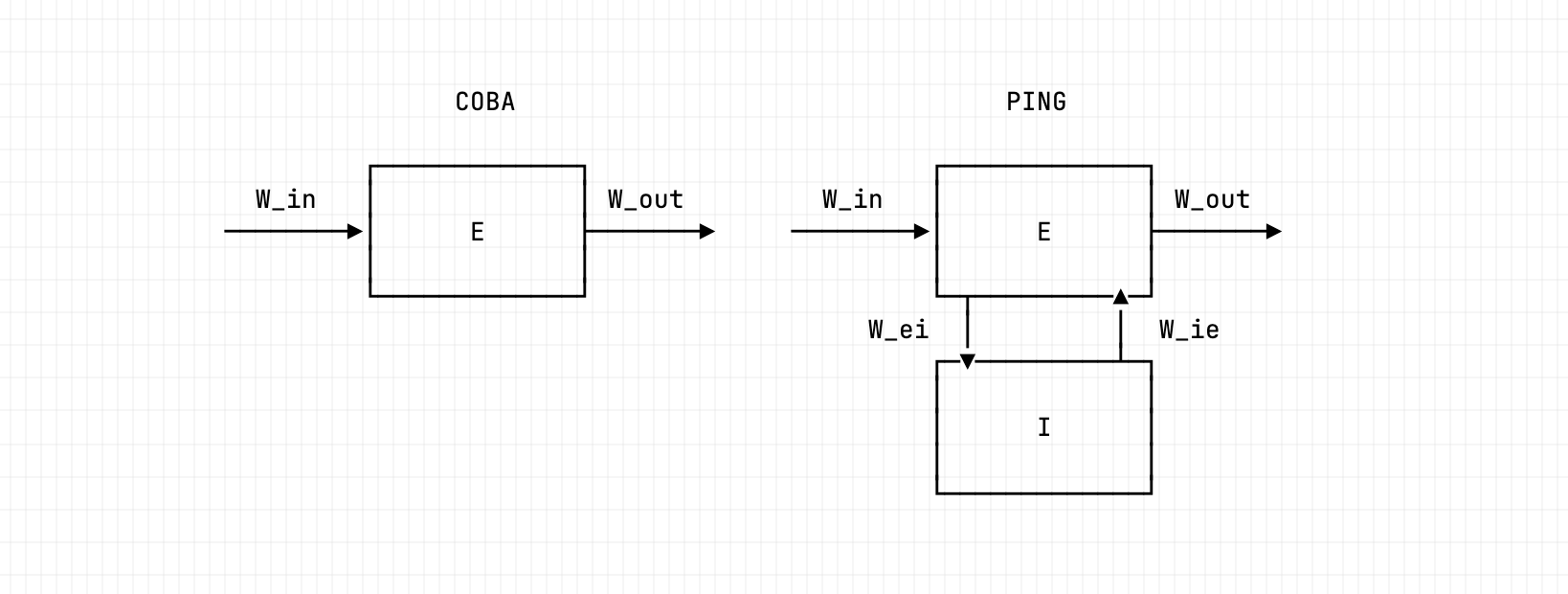
The PING architecture. An input layer drives the excitatory population through ; the E→I→E loop is formed by (E to I) and (I back to E), with no I→I synapse. Disabling the I→E loop (ei-strength 0) recovers the COBA reference; engaging it (ei-strength 1.5) produces the gamma rhythm.
COBA Fundamentals
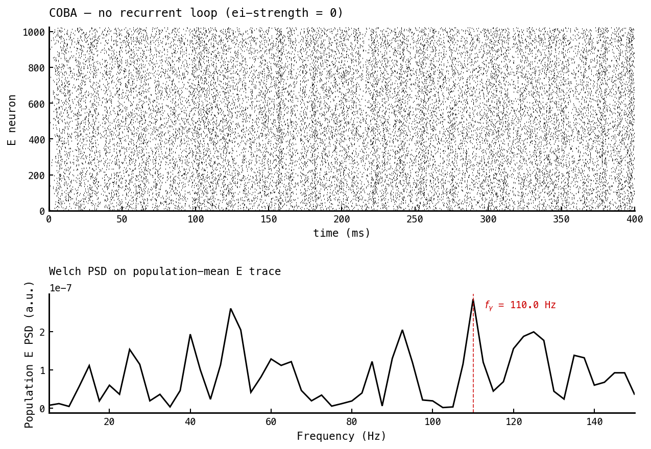
Baseline: recurrent inhibitory loop silent (—ei-strength 0). The E raster fires asynchronously across the full 400 ms; the I population is silent. The Welch PSD on the population-mean E trace shows no isolated gamma peak — only the broadband structure of input-driven asynchronous firing. This is the “PING off” reference.
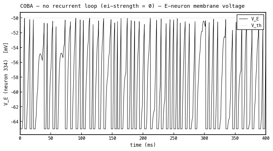
Membrane voltage (black) of the most active E cell, recurrent loop off (COBA, ei-strength 0). Driven only by feedforward input, the cell charges toward threshold ( mV, faint dashed) and hard-resets to mV each spike — irregular, input-paced firing with no rhythmic structure.
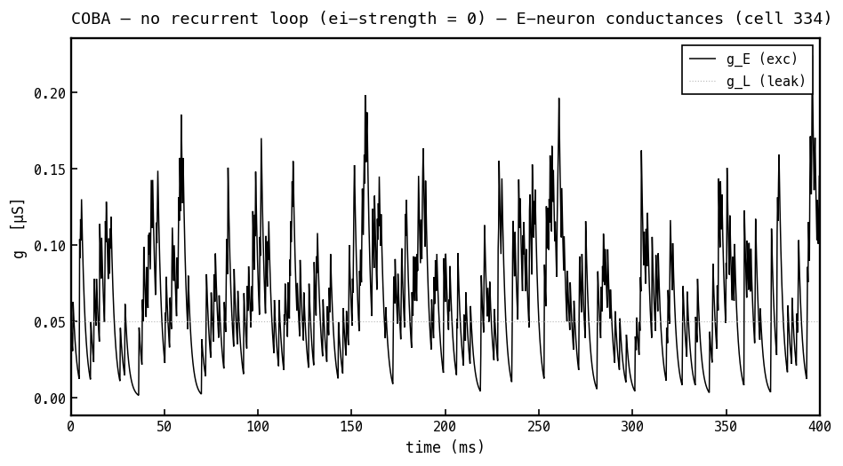
Synaptic and leak conductances on the same E cell, COBA mode. Only the excitatory conductance (black) is active — it steps up with each input spike and decays with — while the leak (faint dotted) is fixed. There is no inhibitory because the I→E loop is off. All conductances are non-negative: they count open channels, not current direction or sign.
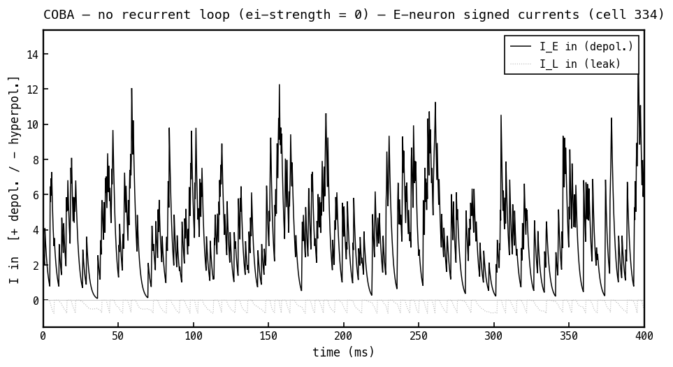
Signed synaptic currents into the E cell, COBA mode, with (positive = depolarising). With no inhibition, the only synaptic current is the depolarising excitatory current (black); the leak current (faint) hovers near zero.
PING Fundamentals
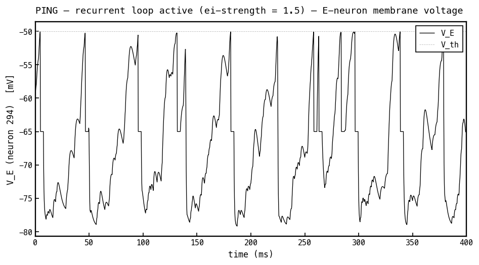
Membrane voltage (black) of the most active E cell, recurrent loop on (PING, ei-strength 1.5), same input as the COBA panel. Rhythmic inhibitory bursts hold the cell below threshold most of the time: each I-burst drags toward mV, and the membrane recovers — and can fire — only as inhibition decays between bursts. The loop turns the irregular firing of Figure 3 into cycle-gated firing.
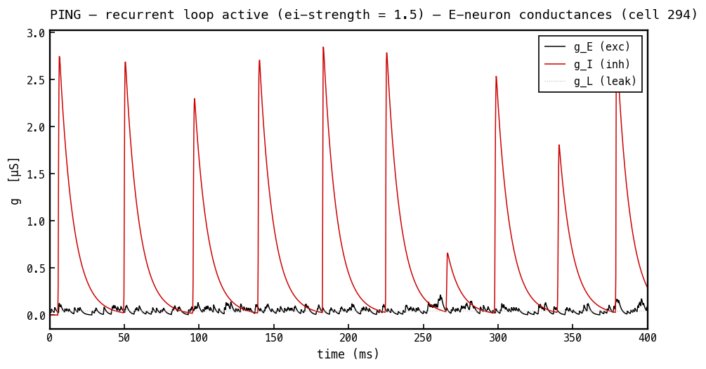
Conductances on the same E cell, PING mode. The inhibitory conductance (red) now dominates — it spikes once per gamma cycle as the synchronous I-burst arrives through , then decays with — while (black) carries the smaller feedforward input and (faint) is fixed. All three traces are non-negative: is large and positive, and that is what shunts the cell — it carries no sign of its own.
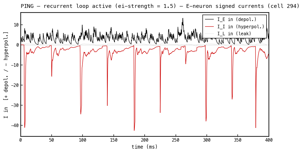
The load-bearing panel. The excitatory current (black) is depolarising. The inhibitory current (red) is negative (hyperpolarising) even though is positive (Figure 7) — the minus sign comes entirely from the driving force whenever sits above mV. The COBA principle made literal: the sign lives in the driving force, never in the conductance.
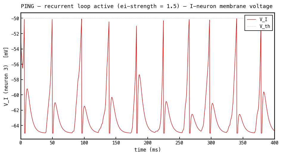
Membrane voltage (red) of the most active I cell, PING mode. The I cell integrates the excitatory volley from the E population and fires once per gamma cycle, so tracks the E-burst envelope — ramping up as E cells fire, crossing threshold, resetting, and waiting for the next volley. This single I-spike per cycle delivers the inhibitory burst seen on the E cell in Figures 7–8.
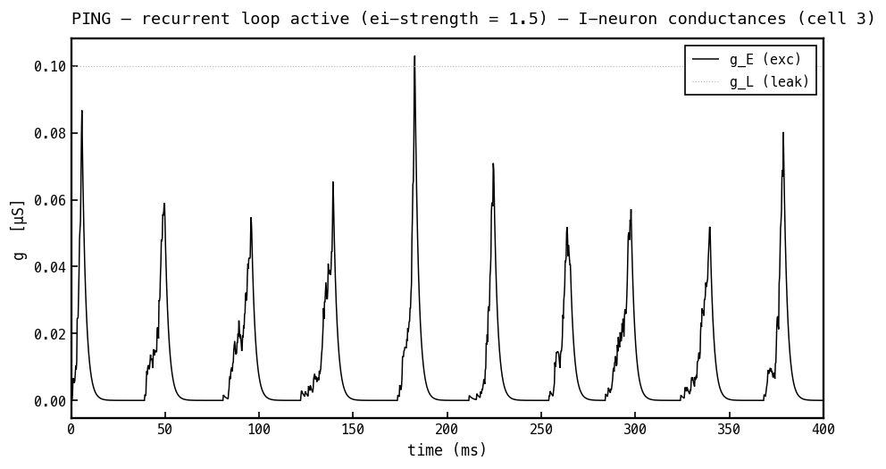
Conductances on the I cell, PING mode. The I cell receives only excitation: (black) is the arriving E-spike envelope (via ) and (faint) is the fixed leak. There is no inhibitory conductance — the architecture has no I→I synapse — which is exactly why the I population can synchronise into the sharp once-per-cycle bursts that clock the loop.
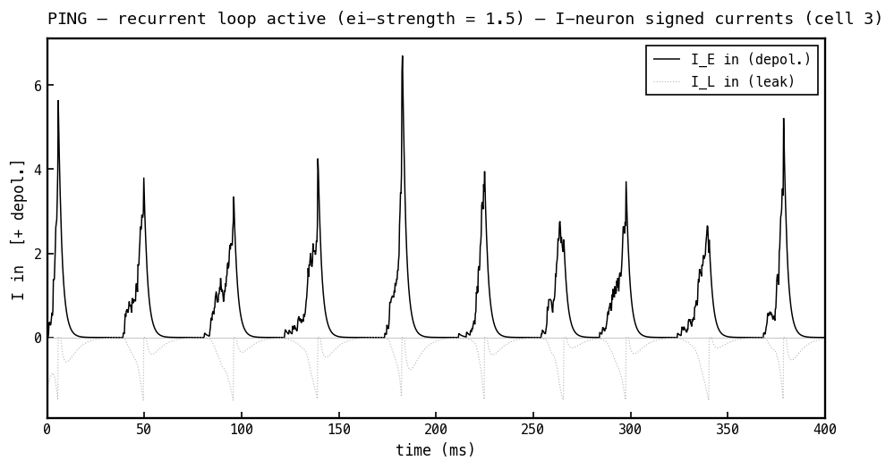
Signed currents into the I cell, PING mode. With no inhibitory input, only the depolarising excitatory current (black) and a small leak current contribute. Read Figures 6–11 together and the loop is in cross-section: E spikes ramp on I (Figures 10–11) → I fires once per cycle (Figure 9) → that spike delivers the inhibitory burst on E (Figure 7) → its negative current shuts E down (Figures 8, 6) → decays → E refires. That delayed E→I→E loop is PING.
Note the harmonics: the Fourier transform of a comb is another comb.
Frequency–current (f-I) curves
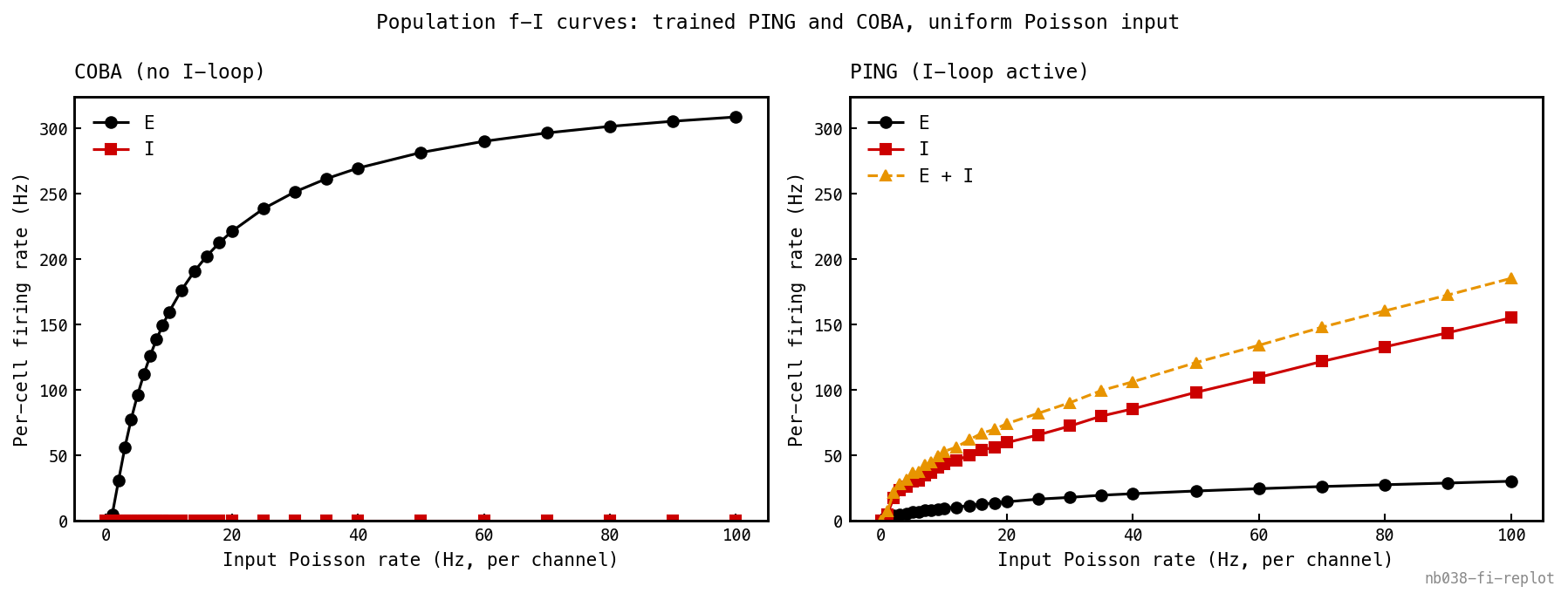
Population f-I curves — mean per-cell firing rate vs input Poisson rate — for trained COBA (left) and trained PING (right) under spatially uniform input (all 784 channels at the same rate, no digit structure), both panels on a shared y-axis. COBA: E (black) climbs steeply and saturates toward its refractory ceiling (≈ 310 Hz at 100 Hz input), I (red) flat at zero. PING: a recruitment cliff at low input, after which E is held ≈ 10× lower than COBA across the range — only ≈ 30 Hz at 100 Hz input. The I curve and E+I total ride above the E curve: I fires harder than E to suppress it. The function of PING — dynamic-range compression, folding drive that would saturate E into a bounded gamma cadence.
Training
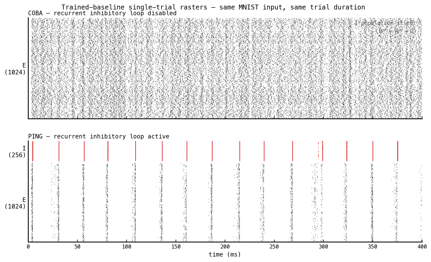
Trained COBA (top, —ei-strength 0) and trained PING (bottom, —ei-strength 1) replayed on the same MNIST digit 0 over 400 ms. Same architecture, same trainable-parameter count, same recipe. Only difference: PING’s recurrent E ↔ I matrices are non-zero. COBA fires asynchronously at ≈ 96 Hz; PING fires in gamma bands at ≈ 28 ms cadence with ≈ 10 Hz mean per E cell, the I population firing synchronous bursts trailing each E-burst.
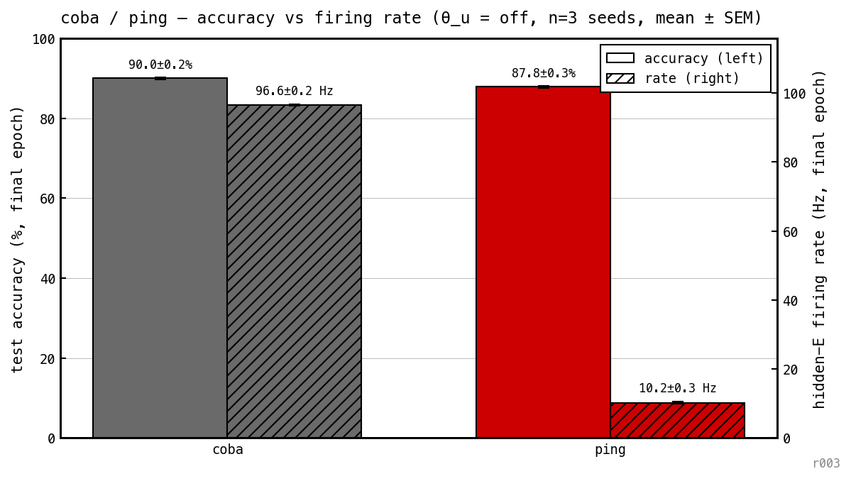
Final test accuracy (solid) and mean hidden-E firing rate (hatched), per model, at the unregularised baseline. PING: 89.33% at 10.20 Hz E rate. COBA: 90.17% at 96.56 Hz E rate — comparable accuracy, ≈ 9.5× fewer E spikes per cell.
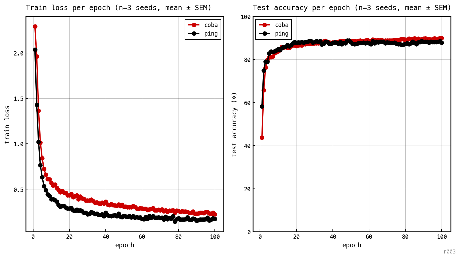
Per-epoch train loss and test accuracy for each baseline model, averaged over three seeds. Both models descend at similar pace and finish within ≈ 0.5 pp.
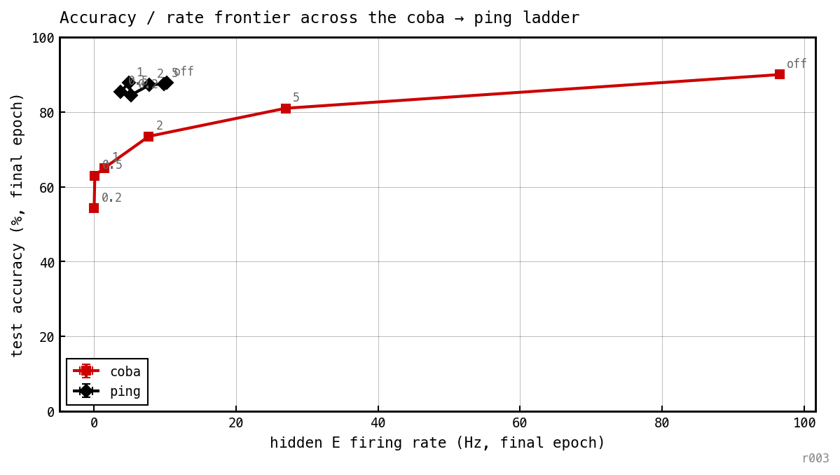
Test accuracy vs achieved hidden-E rate; one point per spike-budget level. COBA traces a curve from ≈ 96 Hz down to ≈ 0 Hz, costing ≈ 28 pp accuracy. PING spans only 3.7–9.9 Hz across every — the penalty has bounded leverage and never pushes the network into COBA’s territory.
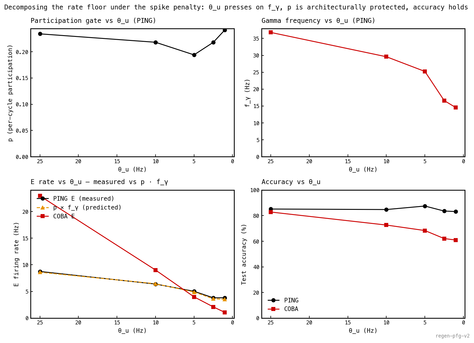
stays in 0.19–0.24 across the entire sweep — the architecture protects the participation gate. slides from ≈ 37 Hz to ≈ 15 Hz as the penalty tightens — the optimiser pushes on the oscillator, not on the gate. The predicted curve overlays the measured E rate within 4%. PING accuracy holds at 83–87%; COBA’s collapses from 83% to 61%.
Near-strict 1 spike per cycle in PING
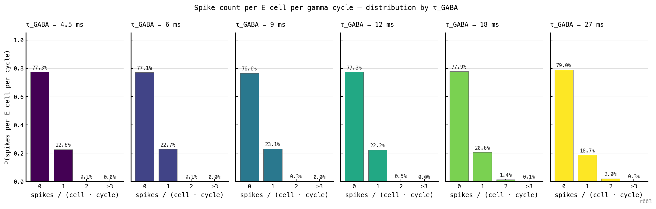
Distribution of E spike count per gamma cycle per cell, by , three seeds aggregated. Across 48 million (cell, cycle) pairs the architecture is overwhelmingly bimodal: each cell emits either zero spikes in a cycle (≈ 77%) or exactly one (≈ 22%). Two-or-more events occur in 0.55% of cycles; three-or-more in 0.04%. The ”≤ 1 spike per E cell per cycle” reading of the affine law is empirically supported — the slope is per-cycle Bernoulli participation, not a phenomenological fit parameter.
Frequency vs
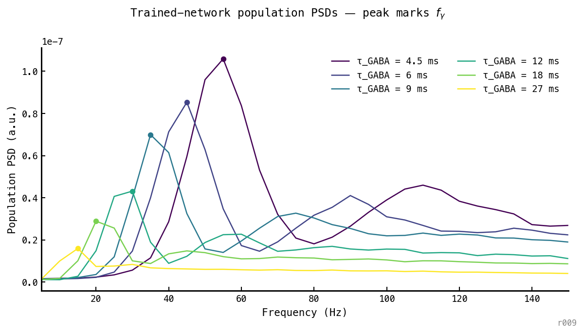
Trial-mean Welch PSDs by . Dots mark the parabolic-interpolated peak. Peak shifts cleanly from ≈ 14 Hz at ms to ≈ 54 Hz at ms; no overlap between adjacent conditions.
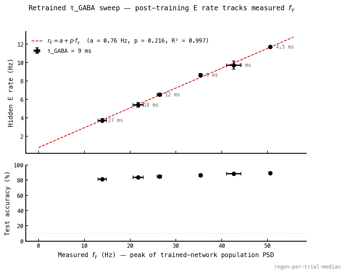
Mean post-training E rate vs , six clusters × three seeds, error bars from seed variance. The affine fit () passes through every error bar. The slope is per-cycle participation; the intercept is a non-rhythmic baseline. Accuracy (bottom) stays flat at 81–89% — the rate change is not paid in classification.
Perturbations
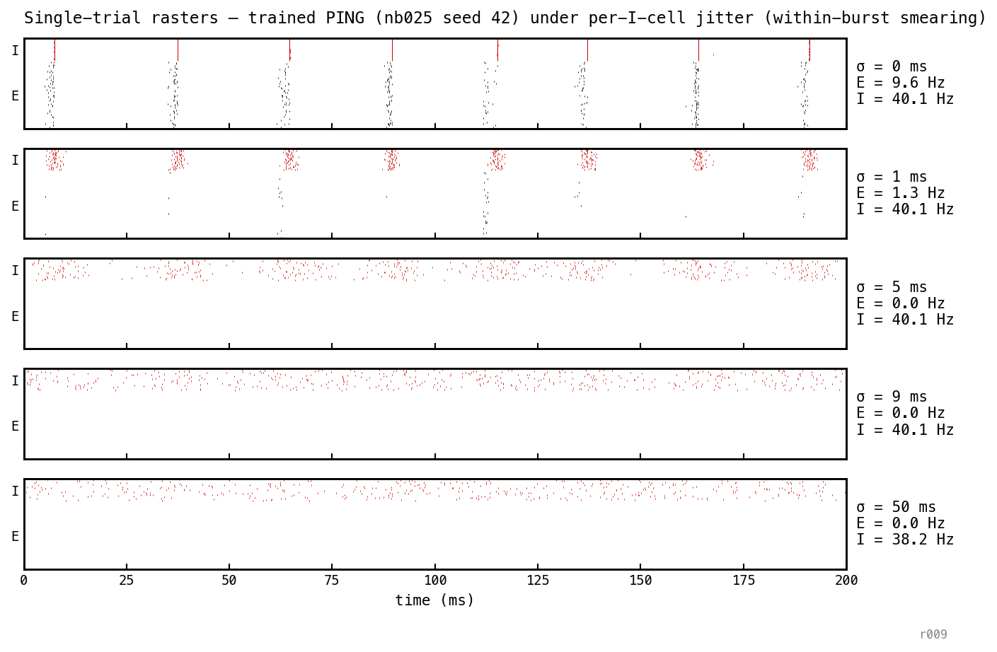
Single trial replayed at five per-cell jitter levels (each I-spike given an independent Gaussian offset; mean I rate preserved). At ms the bursts smear into a few-ms cluster and E firing collapses to 1.6 Hz; at ms the I-stream is a continuous low-variance shunt and E is silenced. Destroying within-burst sharpness silences E.
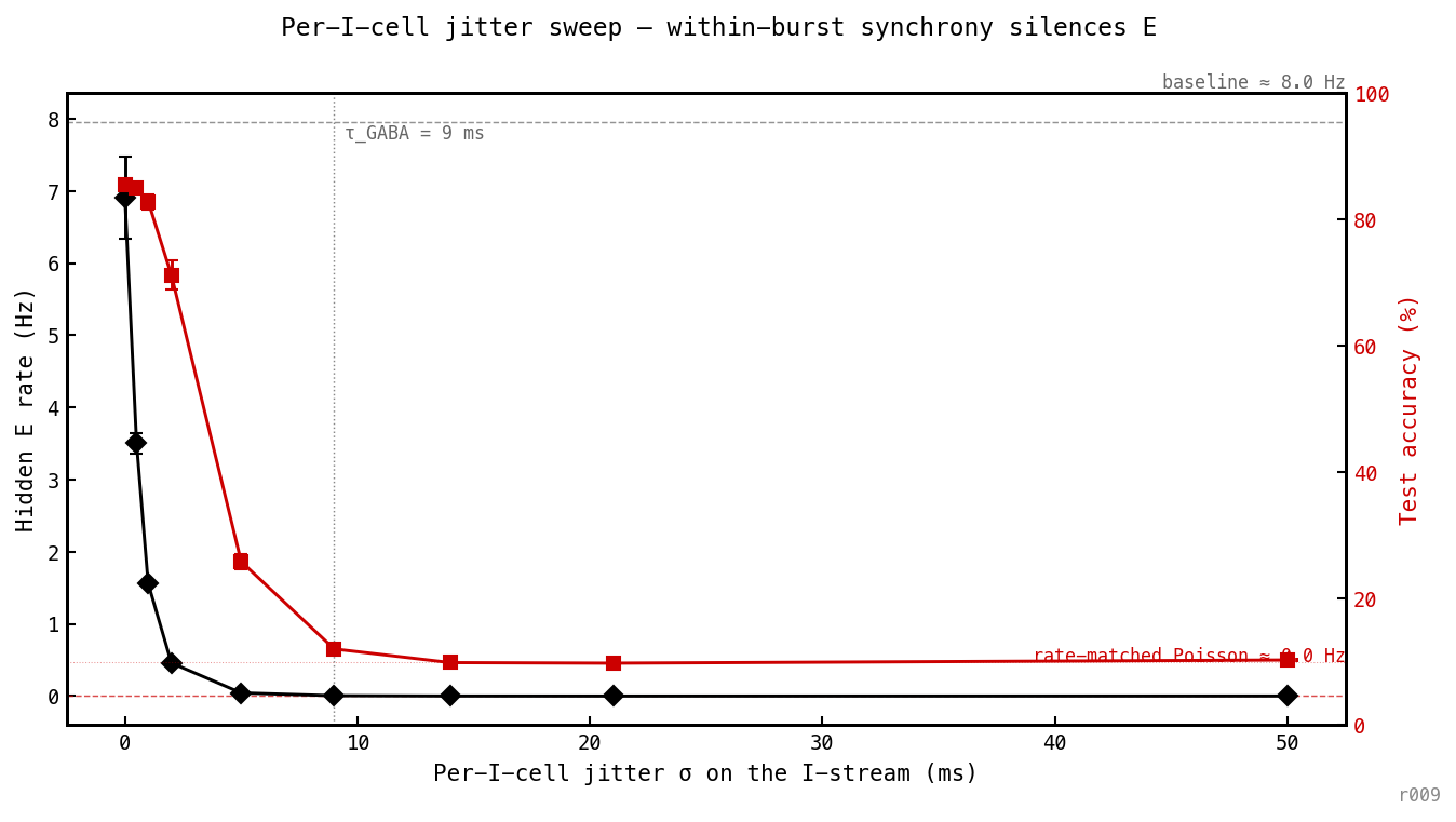
Per-I-cell jitter sweep, three seeds. E rate (left) falls monotonically from baseline — halved by ms — and is essentially zero by ms, well below ms. Accuracy (right) holds at ≈ 85% up to ms then collapses to chance by ms. Within-burst synchrony is a separate axis from burst placement.
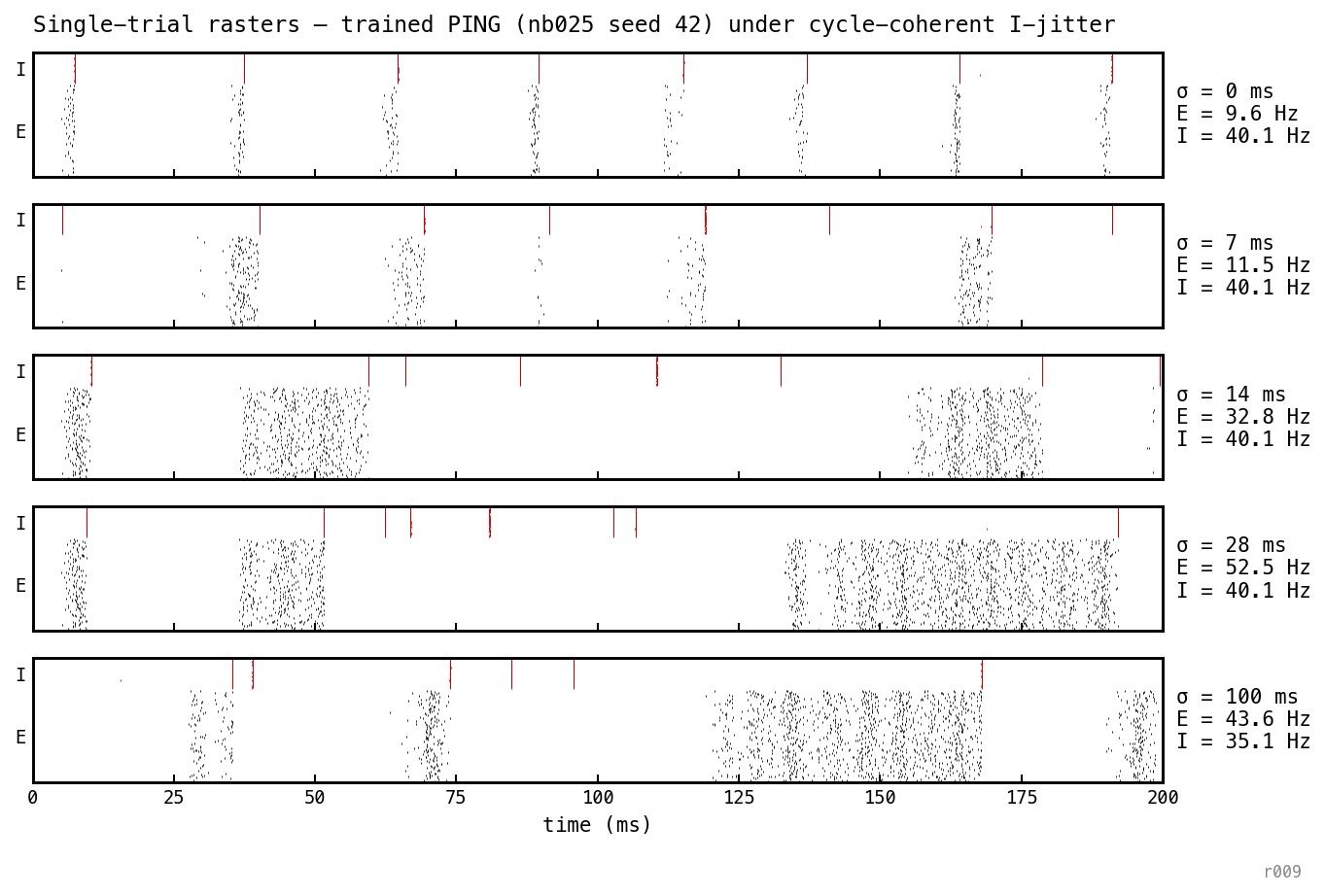
Single trial replayed at five cycle-coherent jitter levels — whole bursts displaced bodily, within-burst synchrony preserved exactly. The I-bands stay vertical and crisp at every ; what changes is where each burst lands. At larger the bursts decouple from the gamma cycle, opening gaps that E fires through.
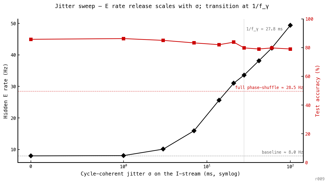
E rate (black) and accuracy (red) vs cycle-coherent jitter . The rate is flat for ms then transitions, crossing the phase-shuffle ceiling (≈ 29 Hz) near the predicted inflection ms (vertical dotted). The operative timescale is the gamma cycle period — destroying burst placement releases E toward COBA territory, while accuracy holds at 79–86%.
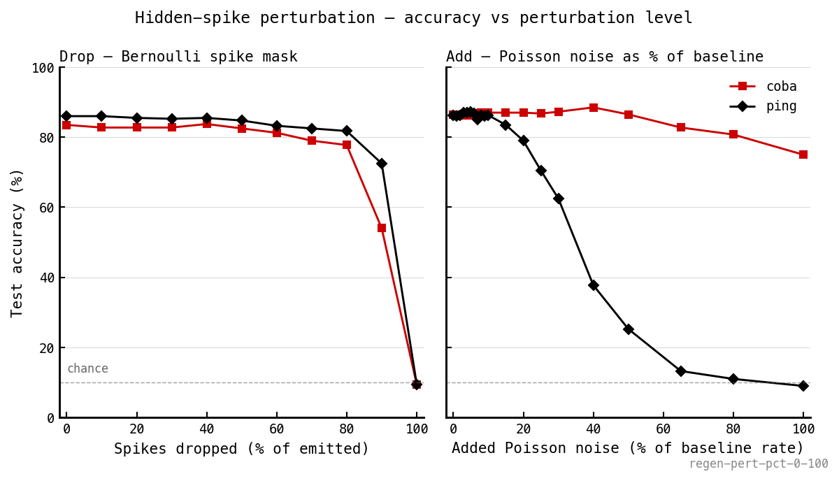
Hidden-spike perturbation of trained PING and COBA at inference (nb037). Left (drop): PING tolerates up to ≈ 80% of emitted spikes dropped — the loop compensates because it weakens proportionally rather than phase-corrupting. Right (add): PING collapses on injected Poisson noise between 15% and 50% of baseline rate, while COBA stays at 75% even with 100% extra. Drops forgiven, adds break the gating — the gamma cycle made visible.
COBA → PING I-loop transfer at inference
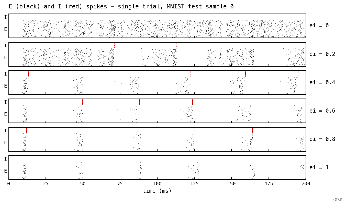
Trained COBA replayed at six inference-time ei_strength values; same trial, same weights, fresh I-loop each row. At ei = 0 the asynchronous-dense COBA pattern persists; by ei ≈ 0.4 the same feedforward weights produce gamma cycles. The PING dynamics come from the inhibitory architecture, not from training.
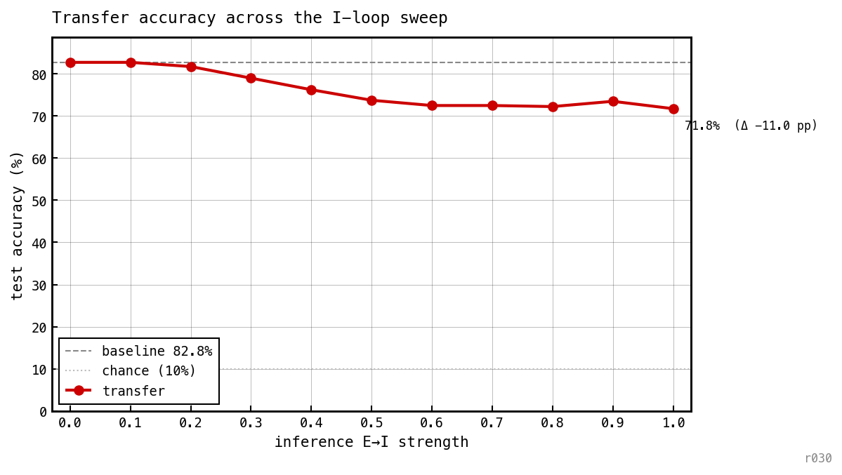
Test accuracy vs inference-time ei_strength on trained COBA weights. Accuracy stays within ≈ 12 pp of the COBA baseline across the full range.
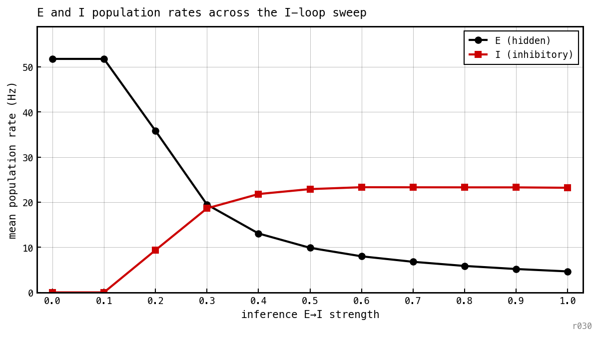
Mean E and I rates across the same ei_strength sweep. E rate falls monotonically from ≈ 52 Hz (ei = 0) to ≈ 5 Hz (ei = 1); I rate rises from zero to ≈ 23 Hz. Suppression is continuous in the loop strength — PING gating is a post-hoc sparsity knob.
Sequential MNIST
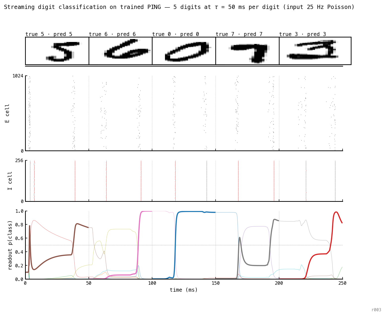
Five sequential digits (5, 6, 0, 7, 3) at ms each — ≈ 2 gamma cycles per digit, 250 ms total, no retraining. Gamma cadence (≈ 28 ms) is preserved across the stream. The readout flips to the new digit within one cycle of each transition and reaches near 1.0 by the segment’s end. 5/5 correct.
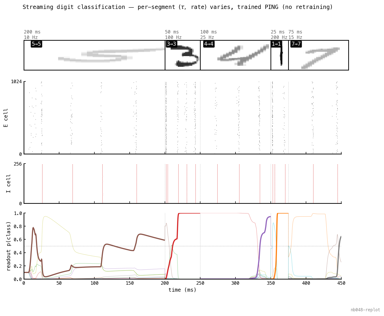
5/5 with varying within a single stream — durations 25–200 ms, rates 10–200 Hz. Thumbnail opacity ∝ input rate. The sliding window uses each segment’s own , so each digit’s prediction respects its presentation window.
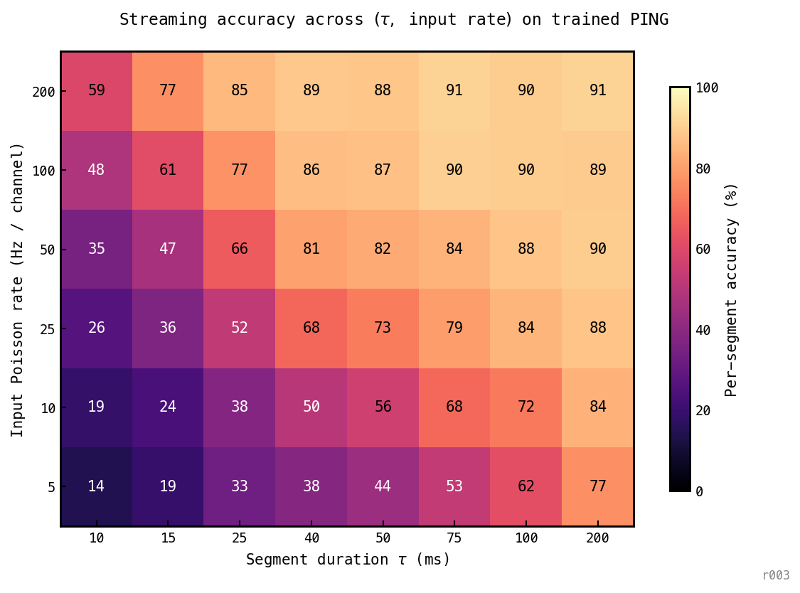
48 cells, 3 seeds × 1200 segments per cell. A sub-cycle failure floor appears below ms — the architecture cannot classify within less than one gamma cycle regardless of drive (the cycle is the temporal quantum). Above it, iso-accuracy contours run diagonal: and input rate substitute for each other, and the trained (200 ms, 25 Hz) operating point sits interior to a broad plateau.
Videos
Drive-threshold scan (nb003). Each frame is a fresh simulation on MNIST digit 0; the stim window multiplies the Poisson input rate by the overdrive factor shown on the frame. Three regimes emerge: async baseline (1–1.2×), unstable PING onset (1.2–6×), and stable PING (6× onwards).
Integration-step scan (nb005), stim-overdrive pinned firmly inside the stable-PING regime so dt is the only knob that can break the rhythm. Stable until about dt = 1.65 ms; beyond that the whole population saturates after PING onset — integrator instability rather than loss of the rhythm.
Constant-drive scan (nb004), companion to nb003 with no stim window — the Poisson input rate is flat across the whole run and the sweep walks that single rate from low to high, mapping PING onset as a function of constant input drive with no transient to confound it.
E→I coupling scan (nb006): with drive held fixed, the E→I coupling strength sweeps from the async baseline through the emergence of gamma as the feedback loop closes. No PING until about E→I strength 1.6, then unstable onset from 1.6 onwards.
Spike movie (nb002): one continuous fixed-network run, no scan. Top: two spike grids — the E population (black) and I population (red), each cell filled if it spiked in that frame’s window. Middle: the raster over the whole run, E in black and I stacked above in red. Bottom: the per-channel input rate, a low → high → low square wave across three equal windows. In the low windows the grids twinkle sparsely and I is dark; in the high window both grids flash in synchronous gamma volleys and the raster locks into bands. The clock ignites when drive crosses threshold and extinguishes within a cycle when it falls — gamma is a property of the loop, gated by drive, not of any single cell.
Works in progress, not presented here.
- When and are trainable, network does not discover PING (nb049).
- Rates dont stabilise across training (nb024).
- Mean field approximation predictions (nb033).
- Rate floor of PING under spike penalty under investigation (nb025).
- Rates vs size of I pool (nb047).
- Rates and accuracy vs and (nb036).