022 — COBA Dale's Law On vs Off
Abstract
Trains COBA twice — once with Dale’s law on the trainable matrix, once off — every other knob held fixed, so any difference is attributable to the constraint alone. The recurrent E–I matrices are fixed buffers either way, so the experiment isolates the trainable-feedforward effect of forcing input projections non-negative.
Methods
Two cells, both running the COBA recipe:
- COBA/dales —
--dales-law(default). The trainable is clamped non-negative at every forward pass. - COBA/no_dales —
--no-dales-law. Signed weights allowed everywhere.
| Parameter | Value |
|---|---|
| Setup | |
| Tier | extra small |
| Dataset | ! mnist (default: scikit) |
| Model | ! ? (default: ping) |
| Architecture | |
| Hidden | ! ? (default: 1024) |
| T | 200 ms |
| dt | ! 0.1 ms (default: 0.25 ms) |
| Input rate | ! ? (default: 25 Hz) |
| Seed | ! 42 (default: —) |
| Training recipe | |
| Samples × Epochs | 100 × 1 |
| Batch size | ! ? (default: 64) |
| Learning rate (η) | ! ? (default: 0.01) |
| cells | ! dales, no_dales (default: —) |
- Recipe. —ei-strength=0 (no active I-loop), —readout=mem-mean, —readout-w-out-scale=100, —lr=0.0004, —w-in=0.3, —surrogate-slope=1, —batch-size=256.
- Same seed (42). The only difference between the two runs is the flag.
Results
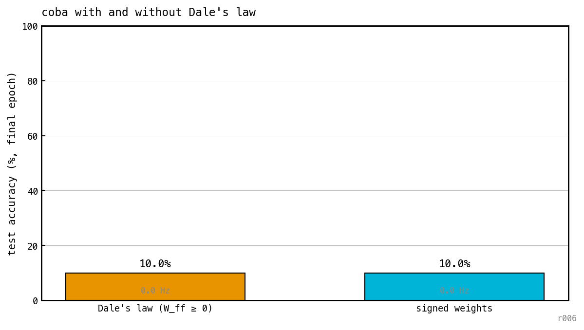
Final-epoch test accuracy under Dale’s law (left) and with signed weights (right). The number beneath each bar is the hidden-E firing rate at the same time point.
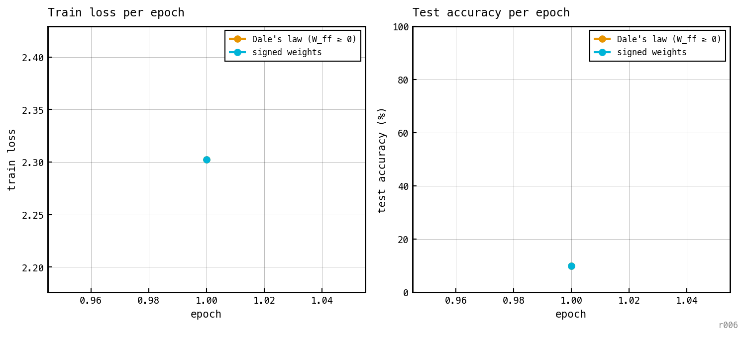
Train loss (left) and test accuracy (right) per epoch, both cells overlaid. Shows how quickly each variant climbs the learning curve and whether the two converge to the same asymptote.
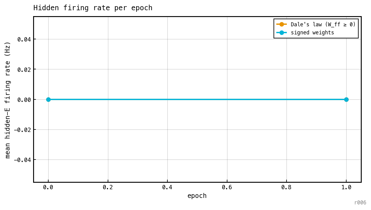
Mean hidden-E firing rate over the training schedule for each cell, including the initial (epoch 0) state. Tells us whether Dale’s law forces a different operating point on the activity, even when end-point accuracy is similar.
![Histogram of all entries of the trained input weight matrix W_ff[0], overlaid for the two cells. Under Dale's law the mass is pinned to non-negative; without it the distribution is roughly symmetric around zero.](/figures/notebooks/nb022/weight_hist.png)
Histogram of every entry of the trained input weight matrix . Under Dale’s law (amber), every entry is non-negative — the optimiser-then-project step pins the mass to the right half-line. Without it (cyan), the distribution sits symmetrically around zero.
Per-cell training videos
COBA reference recipe with —dales-law (default).
COBA reference recipe with —no-dales-law.
Discussion
To fill in after first run. Two things to look for:
- Accuracy gap. Does relaxing Dale’s law buy any task performance? If the constraint is just “free parameters thrown away”, we’d expect signed weights to do slightly better; if the COBA dynamics actually use the sign-fixing (e.g. the cumulative-membrane readout interacts with E vs I), the gap could go the other way.
- Weight-distribution shape. Under Dale’s law, the histogram should be a hard right-half of a distribution. Without it, the distribution should be roughly symmetric — if it isn’t, that tells us the optimiser has discovered an effectively-Dale solution on its own.
Next steps
- Repeat with the ping recipe to see whether the active inhibitory loop changes the conclusion.
- Add a per-population weight breakdown (E units’ inputs vs I units’ inputs) if there’s a meaningful split.
- Pair with 035 — Why PING has a rate floor to ask whether Dale’s law interacts with rate compression.