025 — PING locks E rate ≈10× below COBA (trains)

Abstract

Head-to-head comparison of COBA (recurrent inhibitory loop disabled) against PING (loop active) on MNIST under matched architecture and training recipe. PING locks the hidden E rate to ≈10 Hz while COBA runs at ≈96 Hz; accuracy is within a few points across the two, so the loop buys roughly an order-of-magnitude per-spike economy. The rate-vs-accuracy frontier traced by sweeping the $\theta_u$ rate regulariser shows the floor is structural, not a trade-off the optimiser can navigate away.

Methods

Training recipe (canonical / medium tier):

Parameter	Value
Integration timestep $\Delta t$	0.1 ms
Trial duration $T$	200 ms
MNIST samples (80/20 stratified split of 2000)	1600 train / 400 test ( $\approx$ 2.9% of the 70k-sample MNIST corpus)
Epochs	100

Two configurations of the same COBANet architecture, differing only in whether the E→I→E inhibitory loop is active. COBA (—ei-strength 0) disables the loop; excitatory cells drive each other but receive no structured inhibition. PING (—ei-strength 1) enables the loop, producing pyramidal-interneuron gamma (PING) oscillations at a cadence set by $\tau_\text{AMPA}$ and $\tau_\text{GABA}$ .

Architecture. $N_E = 1024$ excitatory cells, $N_I = 256$ inhibitory cells, single hidden layer. Input: 784 channels (MNIST pixels), Poisson-encoded at 25 Hz peak rate. Readout: mem-mean (time-averaged E spike vector projected through a trained linear layer $W_\text{out}$ ; see ar006 for the full readout specification). Dale’s law enforced.

What is trainable. Only the input weights $W_\text{in}$ ( $784 \times 1024$ , 95% sparse) and the readout $W_\text{out}$ ( $1024 \times 10$ ). The recurrent weights $W_{ee}$ (fixed at zero — Börgers-style PING needs no E→E coupling), $W_{ei}$ , and $W_{ie}$ are initialised once and held requires_grad = False. The synaptic time constants $\tau_\text{AMPA}$ , $\tau_\text{GABA}$ are module-level constants. 813k trainable parameters out of 2.4M total.

Training. Adam, lr = $4 \times 10^{-4}$ , batch size 256, gradient norm clipped to 1.0. Cross-entropy loss on 10-class MNIST (definition in ar006). Gradient stabiliser: —v-grad-dampen 1000 (uniform scaling of per-step voltage gradients). Trial duration $T = 200$ ms at $\Delta t = 0.1$ ms (2000 timesteps).

Tier. Medium: 2000 training samples, 100 epochs, three seeds (42, 43, 44) for baselines, one seed (42) for sweep cells.

Recipe difference. The only parameter that differs between COBA and PING besides —ei-strength is the $W_\text{in}$ initialisation: COBA uses mean 0.3 (std 0.03), PING uses mean 1.2 (std 0.12). PING needs stronger input drive to reliably recruit the I-loop at init.

Results

Trained-network dynamics

Each trained baseline (seed 42, $\theta_u =$ off) is replayed on MNIST digit 0 for 400 ms and the hidden-layer spike trains are recorded.

Two-panel raster figure with shared x-axis (time, 0 to 400 ms). Top panel: trained COBA (recurrent inhibitory loop disabled, ei-strength = 0). Dense asynchronous E firing across all 1024 cells over the entire 400 ms trial; I population labelled silent because W^ei and W^ie are both zero. Bottom panel: trained PING (recurrent inhibitory loop active, ei-strength = 1). E population (1024 cells, black) shows vertical bands at ≈ 28 ms gamma cadence — most cells silent between bursts. I population (256 cells, red, shown above E) shows synchronous bursts trailing each E-burst by a short AMPA delay. 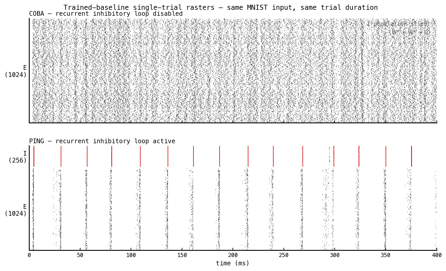— Trained COBA (top, *—ei-strength 0*) and trained PING (bottom, *—ei-strength 1*) replayed on the same MNIST digit 0 input over 400 ms. Same architecture, same trainable-parameter count, same training recipe. Only difference: PING’s recurrent E ↔ I matrices are non-zero. *The visual contrast is the headline of this entry.* COBA fires asynchronously at ≈ 96 Hz; PING fires in gamma bands at ≈ 28 ms cadence with ≈ 10 Hz mean per E cell, and the I population (red, upper region) fires synchronous bursts trailing each E-burst.

Accuracy and firing rate

Final test accuracy and mean hidden-E firing rate are computed for each baseline ( $\theta_u =$ off) across three seeds and reported as means.

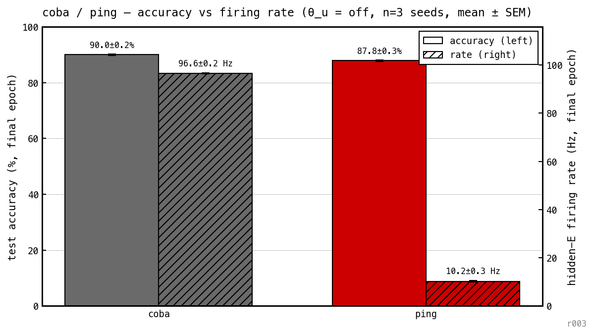
Bar chart: per-model final test accuracy and mean hidden-E firing rate at θ_u = off. — Final test accuracy (solid) and mean hidden-E firing rate (hatched), per model, at the unregularised baseline.

PING: 89.33% at 10.20 Hz E rate. COBA: 90.17% at 96.56 Hz E rate (means over three seeds, 100 epochs). Comparable accuracy, ≈ 9.5× fewer E spikes per cell. Honest scope (nb024 Figure 2): the 9.5× gap holds for the E population only. PING’s I population fires at ≈ 40 Hz to sustain the loop, so PING’s total (E + I) network spike rate is ≈ 49 Hz vs COBA’s ≈ 96 Hz — a 1.6× gap, not 10×. The architecture redistributes the spike budget from broad asynchronous E firing to a concentrated I-burst pattern with cycle-locked sparse E participation, rather than reducing total network spikes. The 10× claim survives if you care about readout-facing spikes (only E projects to $W_\text{out}$ ). The gap does not appear in the loss landscape:

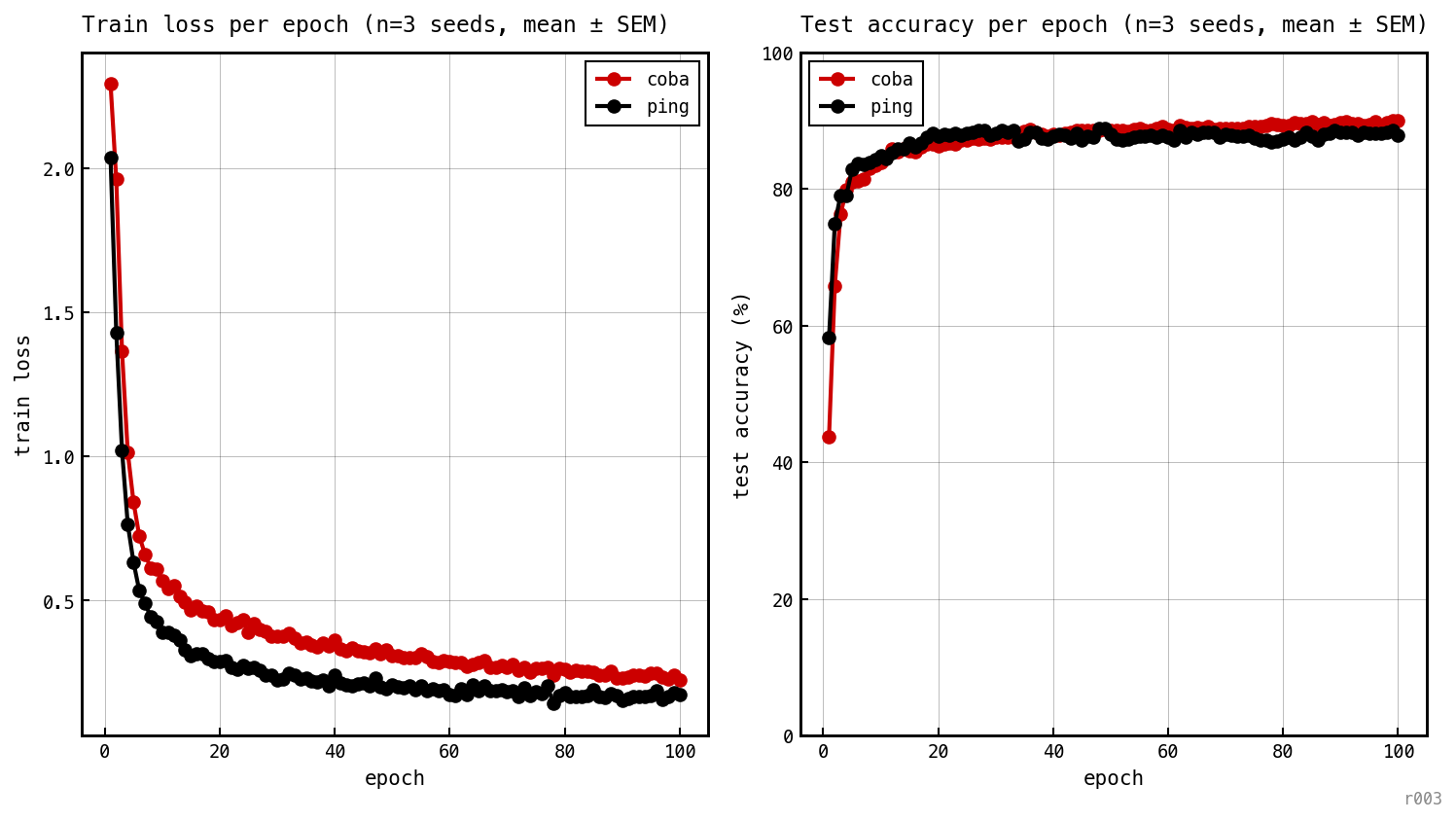
Train loss and test accuracy per epoch, one curve per model at θ_u = off. — Per-epoch train loss and test accuracy for each baseline model, averaged over three seeds.

Both models descend at similar pace and finish within ≈0.5 pp.

The spike-budget control

To probe the rate axis we add a spike-budget regulariser: a soft upper bound on per-trial spike count. For each E cell $n$ , let $\bar z_n$ be the mean spike count per trial. The penalty is

L_\text{rate} \;=\; \lambda \sum_n \mathrm{ReLU}(\bar z_n - \theta_u)^2,

with $\theta_u$ the per-cell budget in spikes/trial and $\lambda = 10^{-3}$ the strength. Only cells whose mean output exceeds $\theta_u$ contribute; cells under budget are free. Total training loss is cross-entropy plus $L_\text{rate}$ .

We sweep six target levels (off, 5, 2, 1, 0.5, 0.2 spikes/trial; at $T = 200$ ms that’s no penalty, 25, 10, 5, 2.5, 1 Hz). Twelve cells, one point per (model, $\theta_u$ ) in (rate, accuracy) space:

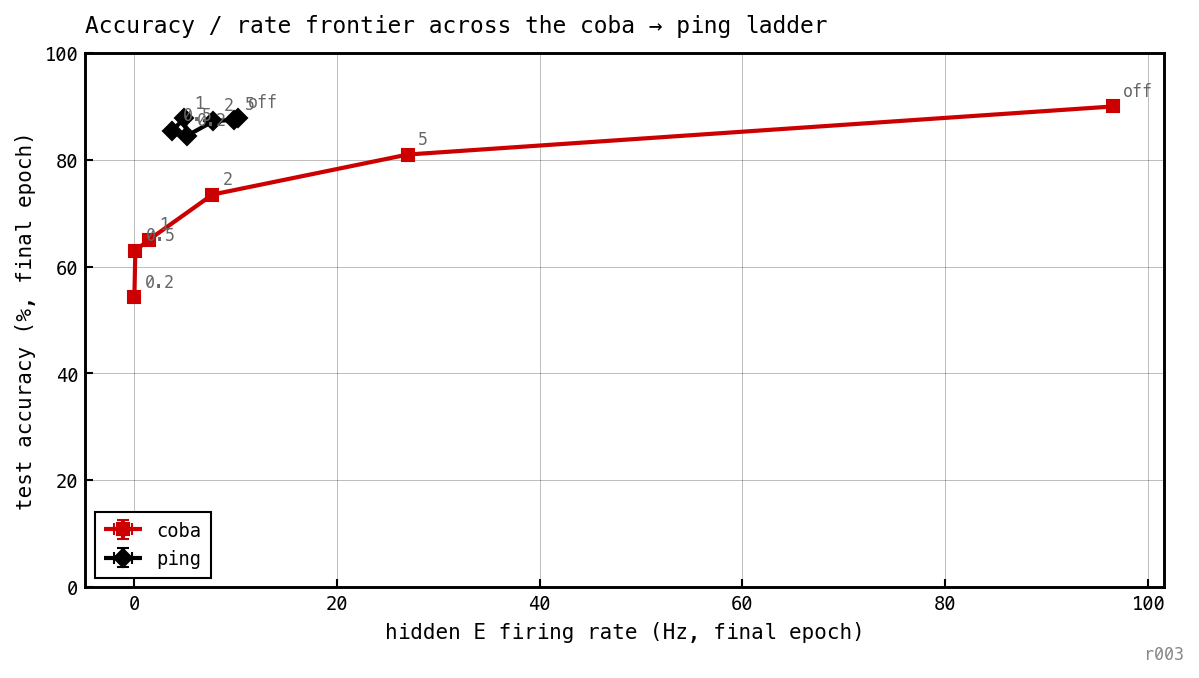
Test accuracy vs hidden-E firing rate, one curve per model; each point one (model, θ_u). — Test accuracy vs achieved hidden-E rate; one point per cell. Gray point labels indicate the spike penalty.

COBA traces a curve from ≈ 96 Hz down to ≈ 0 Hz, costing ≈ 28 pp accuracy (90 → 62%). PING spans 3.7–9.9 Hz across every $\theta_u$ — the penalty has measurable but bounded leverage (9.85 → 3.73 Hz from $\theta_u =$ off to $\theta_u = 0.5$ , ticking up to 5.16 Hz at the tightest $\theta_u = 0.2$ ), and never pushes the network into COBA’s territory.

Decompose the floor into its two factors. The affine law $r_E = p \cdot f_\gamma$ (nb041, nb046) says the rate is the product of per-cycle participation $p$ and cycle frequency $f_\gamma$ . Measure both at every $(\text{model}, \theta_u)$ cell — $f_\gamma$ from the Welch PSD peak of the E-population trace, $p$ via I-burst peak detection and per-(cell, cycle) spike counting in the style of nb046:

Four-panel decomposition vs θ_u (Hz, x-axis inverted so tightest penalty sits at the right). Top-left: per-cycle participation p stays in the 0.19–0.24 band across the entire θ_u sweep for PING. Top-right: gamma frequency f_γ drops smoothly from ≈ 37 Hz at the loosest penalty to ≈ 15 Hz at the tightest. Bottom-left: PING measured E rate (black) overlays p × f_γ predicted (amber dashed); COBA E rate (red) climbs from ≈ 1 Hz at the tightest penalty to ≈ 23 Hz at the loosest. Bottom-right: PING accuracy holds at 83–87% across the entire sweep; COBA accuracy falls from 83% to 61%. 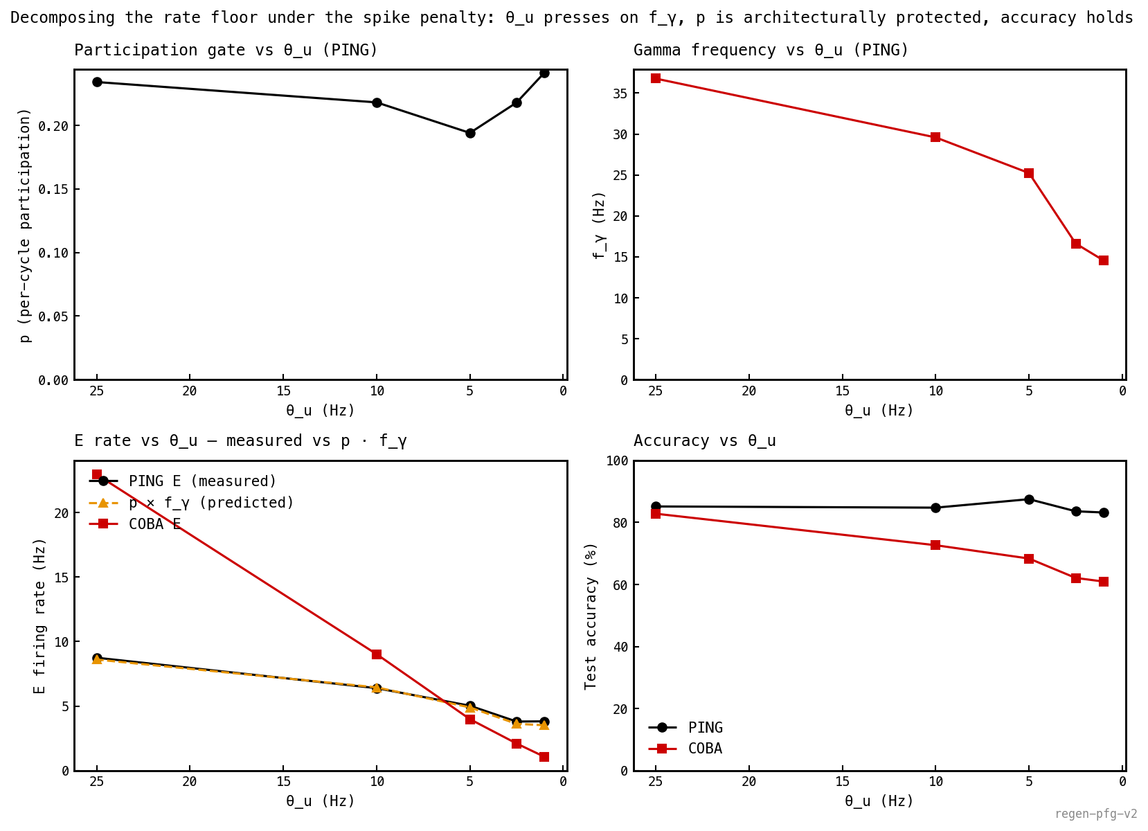— Six $(\text{PING}, \theta_u)$ cells, 256 test trials each. **$p$ stays in 0.19–0.24** across the entire sweep — the architecture protects the participation gate. **$f_\gamma$ slides from ≈ 37 Hz to ≈ 15 Hz** as the penalty tightens — the optimiser pushes on the oscillator, not on the gate. The amber dashed $p \cdot f_\gamma$ predicted curve overlays the measured E rate within 4% across all six cells; the rate change is entirely in $f_\gamma$ . PING accuracy holds at 83–87% the whole way; COBA’s collapses from 83% to 61%.

This rewrites the mechanism: $\theta_u$ lowers $r_E$ by shrinking $W_\text{in}$ , which weakens E→I drive, which slows the gamma oscillator. The participation gate $p \approx 0.20$ never moves; gradient descent cannot touch it. The rate floor in Figure 4 is the cliff that appears when $f_\gamma$ can no longer be driven slower without breaking the loop entirely.

Discussion

Why PING has a rate floor

Figure 4 shows COBA spanning $\geq 2$ decades under $\theta_u$ (≈ 96 → ≈ 0 Hz) while PING moves within a narrow band (9.9 → 3.7 Hz). Three cases, by where the budget sits relative to PING’s ≈ 10 Hz trained rate. (A) No budget: network sits at the gamma-locked attractor. (B) Budget above 7 Hz: penalty inactive at the operating point, equivalent to (A). (C) Budget below 7 Hz: the interesting case — the penalty wants a rate PING cannot deliver, and PING with the loop disengaged is structurally COBA, so why not slide down COBA’s curve toward 0 Hz?

Let $f$ be the recruitment fraction (share of E cells crossing threshold per cycle) and $f^\star$ the critical value at which the I-population fires reliably: $f > f^\star$ engaged PING, $f < f^\star$ a low-rate COBA-like regime. Figure 6 trains four PING networks across this threshold, $W_\text{in}$ initialised at 0.05, 0.1, 0.3, and 1.2 (the standard init).

Two rows by four columns of panels. Each column is one --w-in init (0.05, 0.1, 0.3, 1.2). Top row shows per-epoch test accuracy climbing from chance to ~83%. Bottom row shows per-epoch test-set E (black) and I (red) firing rates: at w_in=0.05 and 0.1 the I rate is near zero for the first epoch or two then rises to ~10 Hz; at w_in=0.3 the I rate is zero for one epoch then rises; at w_in=1.2 the I rate is positive from epoch 1. 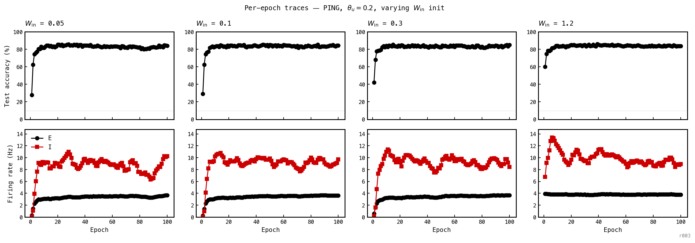— Per-epoch training traces from four PING networks (seed 42, $\theta_u = 0.2$ from epoch 0), one per column. Top: test accuracy. Bottom: test-set E (black) and I (red) firing rates. At $W_\text{in} = 0.05$ and $0.1$ the I population is silent for the first one to two epochs; once $W_\text{in}$ crosses $f^\star$ the loop engages and the network locks into PING. Final accuracies: 84.0% / 84.5% / 85.0% / 83.75%; final I rates: 11.1 / 15.5 / 6.9 / 16.7 Hz.

All four converge to PING within a few epochs. Even $W_\text{in} = 0.05$ — an order of magnitude below the standard init — finds the basin by epoch 2. The basin is attractive from both sides; the floor is structural, not a path-dependence artefact.

To probe the loss landscape directly, scale each trained network’s $W_\text{in}$ by $s \in [0.05, 3]$ at inference, readout frozen. Metrics averaged over the full test set (≈400 samples) at each $s$ .

Six panels showing CE loss, spike-budget penalty, total training-objective loss, accuracy, E rate, and I rate vs W_in scale s, swept at 24 points in [0.05, 3]. Two curves: COBA (red squares) and PING (black circles), both trained at θ_u = 0.2. PING CE drops smoothly across the recruitment cliff near s ≈ 0.3–0.7; PING penalty is small and grows mildly with s. COBA penalty is essentially zero up to s ≈ 1 then explodes (y-axis clipped at 4). PING total loss has a broad minimum near s = 1; COBA total loss has a minimum near s = 1 then climbs steeply. Vertical dashed line at s = 1 marks the trained operating point; vertical dotted line marks ≈f*, the smallest s where the I population first fires. — Inference-time $W_\text{in}$ scale sweep on the two networks trained under the heaviest penalty ( $\theta_u = 0.2$ ). Every $W_\text{in}$ weight is multiplied by a common scalar $s$ ; readout and other weights frozen. 24 values of $s \in [0.05, 3]$ . Top row: CE loss, spike-budget penalty $L_\text{rate}$ , training-objective loss CE + $L_\text{rate}$ . Bottom row: test accuracy (chance dotted), E rate, I rate. PING black, COBA red. Vertical dashed line at $s = 1$ marks the trained operating point; dotted line marks $\approx f^\star$ (PING’s recruitment cliff). Loss panels clipped at 4 — COBA’s penalty reaches ≈32 at $s = 3$ (rate $^2$ scaling).

Three pieces hold the floor in place. First, PING and COBA are different statistical regimes: PING fires in gamma-coordinated bursts at ≈ 36 Hz with ≈ 20% of E cells per cycle (nb046 measured median participation 0.20 directly; mean rate ≈ 10 Hz); COBA fires asynchronously at ≈ 96 Hz with most cells participating. $W_\text{out}$ specialises on whichever regime training produced. Second, the recruitment cliff at $f^\star$ (Figure 7, dotted line at $s \approx 0.42$ ): below it the loop disengages and CE rises to chance — PING’s readout can’t decode the sparse uncoordinated pattern. Third, above the cliff the rate is set by gamma physics: cycle period scales with $\tau_\text{GABA}$ , and at the trained value (9 ms) the natural per-cell rate is ≈5–7 Hz. The penalty can nudge down within the basin, but the engaged loop sets a soft minimum. The total loss has a broad minimum at $s = 1$ : below, the cliff kicks CE up; above, the penalty grows. The ≈2.8–3.5 Hz floor is where the two pressures cross.

PING cannot slide down COBA’s curve to 0.2 Hz for two reasons. Different readouts: Figure 7’s COBA curve shows what 0.2 Hz looks like with a COBA-trained readout (rate ≈1 Hz, CE 2.27, accuracy 53.75%) — its readout was trained on sparse asynchronous firing, PING’s on gamma-coordinated participation; abandoning the cycle breaks the readout. The architecture forbids it: only $W_\text{in}$ and $W_\text{out}$ are trainable; $W^{EI}$ and $W^{IE}$ are fixed at construction, $W^{EE} = 0$ . No setting of the trainable weights suppresses the I-loop. The COBA-low solution lives in the parameter space —ei-strength = 0 opens.

This also explains Figure 6’s universality: at $W_\text{in} = 0.05$ the network starts silent, not COBA-like — too little drive to fire. The only gradient pulls $W_\text{in}$ up; the moment drive crosses $f^\star$ , the fixed E↔I wiring self-assembles the gamma cycle. The optimiser never chose PING; the architecture forced it.

One further observation: PING’s CE drops much more steeply across the recruitment threshold than COBA’s (≈2.30 → ≈0.91 across a factor of 2 in $s$ , vs COBA 2.30 → 2.04 over the same range). The gamma cycle concentrates the class signal — each burst is a structured class-discriminative event, so 2–3 bursts per trial produce a clean readout contribution. COBA’s asynchronous spikes each add a noisy single-cell increment; the signal only emerges after many accumulate. PING does not just use fewer spikes, it uses them more efficiently.

In one sentence: the rate floor is the equilibrium of gamma-cycle dynamics (lower bound set by $\tau_\text{GABA}$ ) and the rate $^2$ penalty (upper pressure), confined to the basin in $W_\text{in}$ -space where $W_\text{out}$ still decodes the participation pattern.

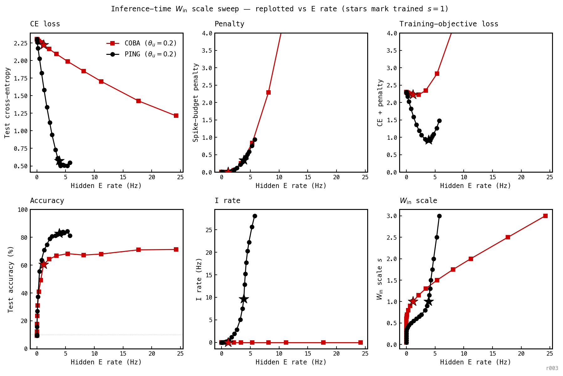
Six panels showing CE loss, spike-budget penalty, total training-objective loss, accuracy, I rate, and W_in scale s, all plotted with hidden E rate (Hz) on the x-axis. Two curves: COBA (red squares) and PING (black circles), both trained at θ_u = 0.2. A filled star on each curve marks the trained operating point at s = 1. — The same 24-point sweep as Figure 7, re-projected with hidden E rate on the x-axis. Filled stars mark each cell’s trained operating point ( $s = 1$ ): PING at $E \approx 3.8$ Hz, COBA at $E \approx 1.0$ Hz. PING’s accuracy reaches its plateau by $E \approx 3$ Hz; COBA climbs slowly and only reaches ≈70% even at $E \approx 28$ Hz.

Next steps

nb036 directly perturbs the recruitment cliff by varying the E↔I coupling, both at inference and during training.
nb037 tests the dynamical character of the floor by perturbing the spike stream (drop, Poisson add, $\tau_\text{GABA}$ sweep).
nb038 runs functional probes (input-rate sweep, COBA→PING transfer, readout latency) on the trained baselines.