036 — W^EI sets the cliff; W^IE shapes the basin (trains)
Abstract
Maps the (wEI, wIE) coupling plane: which weight controls the recruitment cliff, and where do trained networks land when initialised across it? wEI moves the cliff (E→I drive is the recruitment knob); wIE shapes the basin above engagement but does not move the cliff. Training from each grid point lands in two distinct basins — a low-E PING corner and a high-E silent-I stretched-COBA corner.
Methods
Training recipe (canonical / medium tier):
| Parameter | Value |
|---|---|
| Integration timestep | 0.1 ms |
| Trial duration | 200 ms |
| MNIST samples (80/20 stratified split of 2000) | 1600 train / 400 test ( 2.9% of the 70k-sample MNIST corpus) |
| Epochs | 10 |
PING and COBA baseline definitions, training recipe, and the spike-budget regulariser are in nb025. The recruitment cliff at is introduced in nb025. This entry asks: which part of the E↔I coupling architecture controls the cliff’s position, and what happens when we train the network from coupling initialisations spanning both sides of it?
Results
Coupling sweep: shifting the recruitment cliff
If is set by the E↔I coupling, altering or at inference should move it. On the trained PING baseline ( off), we multiply either or by a scalar in and re-run the scale sweep on top. All other weights frozen.
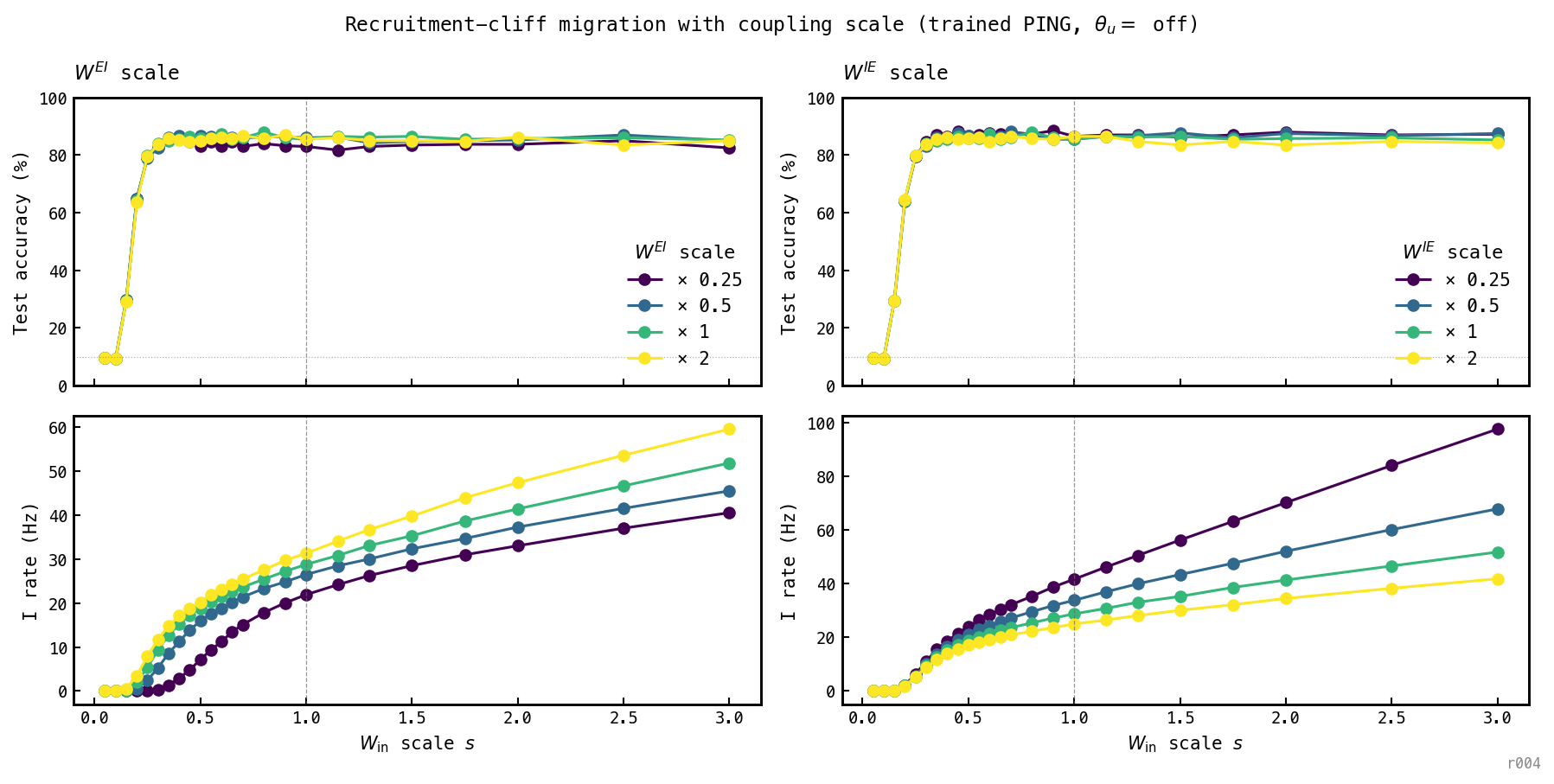
Inference-time scale sweep on trained PING ( off) with either or scaled. Top: accuracy. Bottom: I rate. Left: sweep, fixed. Right: sweep, fixed.
Figure 1 cleanly separates the two roles. moves the cliff (left column): halving E→I coupling shifts the recruitment edge from to , quartering it to . Doubling does not push it further left because below the feedforward drive itself is too weak to make E fire — the bottleneck has moved from I-cell recruitment to E-cell firing, and stronger cannot rescue silent E spikes. does not move the cliff (right column): all four curves lift off at , because only matters once I has fired, and at the cliff I has not. Above the cliff the right-column I-rate curves separate visibly — stronger inhibition per I spike suppresses the steady-state I rate. So the recruitment threshold is set by the E→I drive; inhibitory feedback shapes the basin only above engagement.
The scaling has a clean quantitative signature: the unsaturated points obey to three significant figures (products 0.250, 0.247, 0.250), so empirically rather than the naive . The exponent is a fingerprint of the gain function near rheobase, and a concrete prediction for the mean-field analysis in nb033 to reproduce.
x training grid
The coupling-sweep results above scaled and on an already-trained network. A stronger test is to train one network per grid point with and initialised to specified values from scratch, under heavy spike penalty. Do the resulting solutions cluster into a PING-like region and a COBA-like region?
Method: 5×5 grid over (mean initialisation, std fixed at mean). One PING-architecture training run per cell at from epoch 0, (a compromise between COBA’s 0.3 init and PING’s 1.2 — gives the no-loop cells a fair shot at converging), 100 training epochs per cell, seed 42. All other hyperparameters from the standard PING recipe. 25 trainings on Modal A100 in parallel. Reporting per-cell best-epoch accuracy.
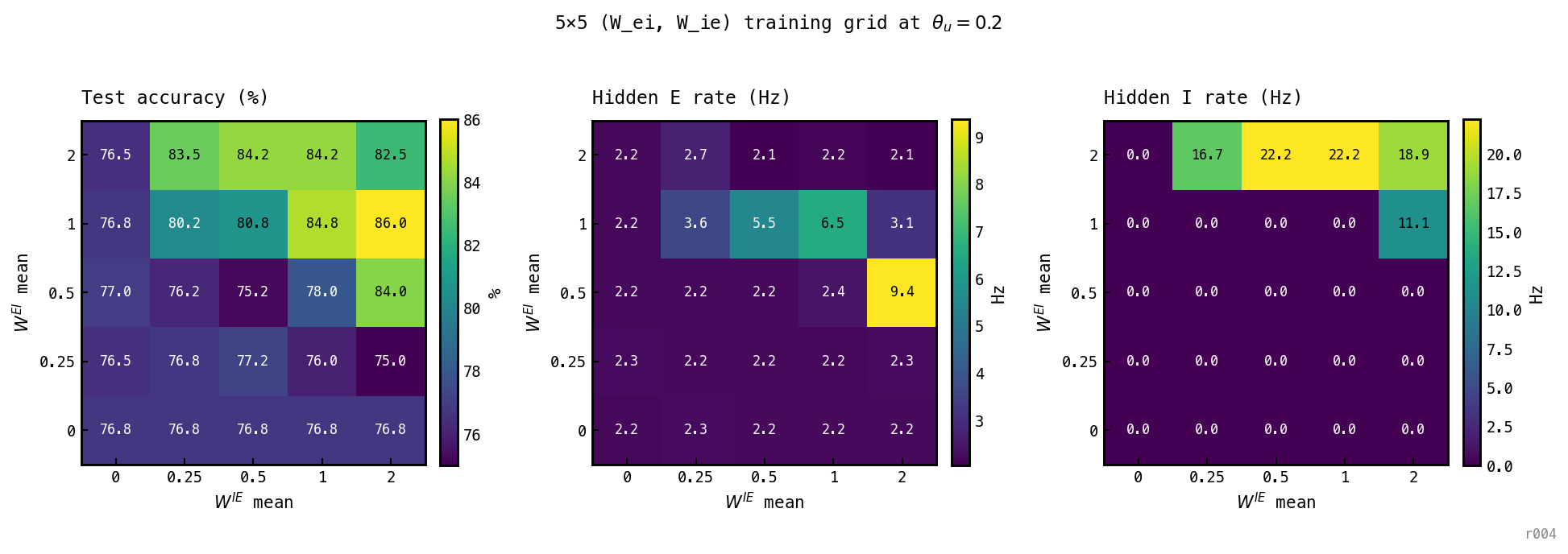
Three heatmaps on the 5×5 () training grid. One PING-architecture network per cell, trained from scratch at for 100 epochs, . Left: best-epoch test accuracy. Middle: hidden-E rate. Right: hidden-I rate (the cluster discriminator).
Three regions emerge:
- No-loop band ( row OR column): accuracy ≈ 76.5–77%, E rate 2.2 Hz, I rate 0. Without a closed E→I→E loop the optimiser settles at the same COBA-low operating point regardless of which side of the loop is zero — the structural-equivalence prediction holds.
- PING cluster ( with , plus the entire row from ): I rate 11.1–22.2 Hz, E rate 2.0–3.6 Hz, accuracy 80.25–86.0%. Gamma signature; the recipe baseline at peaks at 86.0%, and the cluster includes the over-inhibited corner at 82.5% — only ≈ 3.5% drop from peak.
- Stretched-COBA cluster ( with most , plus and ): I rate 0, E rate 2.2–9.4 Hz, accuracy 75–84%. The I-loop never engages; the optimiser uses pure E-cell firing to fit the digits. The high end of this cluster is the cell at — at 84.0% with E = 9.37 Hz and I = 0, the I-loop is silent yet accuracy is within 2 pp of PING peak.
The cell deserves special attention. With 30 epochs of training it sat in the PING cluster (some seeds engaging I, some not). At 100 epochs the optimiser deterministically finds a no-I, high-E solution (E = 9.37 Hz, I = 0, acc = 84%). This is a new attractor that the shorter-training version masked — the network learns to classify with elevated E firing in lieu of recruiting the loop.
The clustering confirms the GH #29 hypothesis: under heavy spike penalty, the (coupling, accuracy, rate) outcome lands in qualitatively different solutions depending on coupling strength. The recruitment cliff that the inference-time coupling sweep located (Figure 1) is reproduced here as the boundary of the PING cluster at (with ). The no-loop band at 76.5–77% sits ≈ 9 pp below PING’s 86% peak — substantially better than chance, but the loop is a real accuracy advantage even at this spike budget. The diagonal slice below walks this transition at higher resolution along the canonical line.
Plotting the same 25 cells in (E rate, accuracy) space — colour-coded by I rate — makes the cluster structure direct:
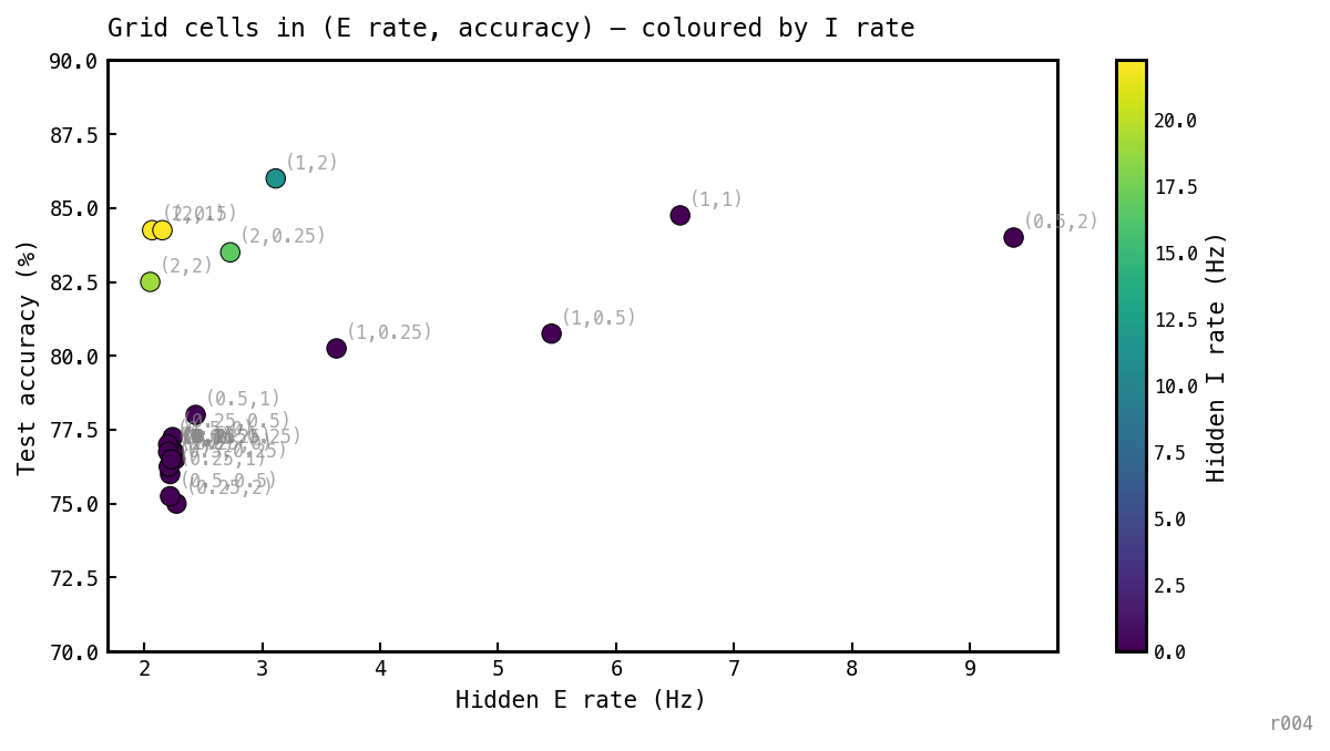
Each dot is one cell of the 5×5 training grid, plotted at its best-epoch test accuracy vs final hidden-E rate. Colour encodes the third quantity — hidden-I rate — which is what discriminates the clusters. Labels are .
Two clouds separate in this view. Dark-purple points (I rate ≈ 0) span accuracy 75–84% with E rates 2.2–9.4 Hz — the no-loop / stretched-COBA region. The top of this band is at 84% with E = 9.4 Hz, the high-accuracy E-only solution: silent I, elevated E rate, accuracy within ≈ 2 pp of the PING cluster. Yellow/green points (I rate > 11 Hz) sit above at 80–86% accuracy with E rates clamped to 2–3.6 Hz by the active inhibitory loop — the PING cluster, distinguished from no-loop by lower E and active I.
The vertical gap between the two clouds is the recruitment cliff measured in accuracy units: ≈ 2–6 pp depending on where you draw the comparison. The high-E no-loop attractor at closes most of that gap with E firing alone, but at 4× the per-cycle E spike count.
Overlaying the COBA and PING -sweep frontiers (Figure 5 of nb025) directly onto the same axes pins where the grid solutions live relative to the two canonical baselines:
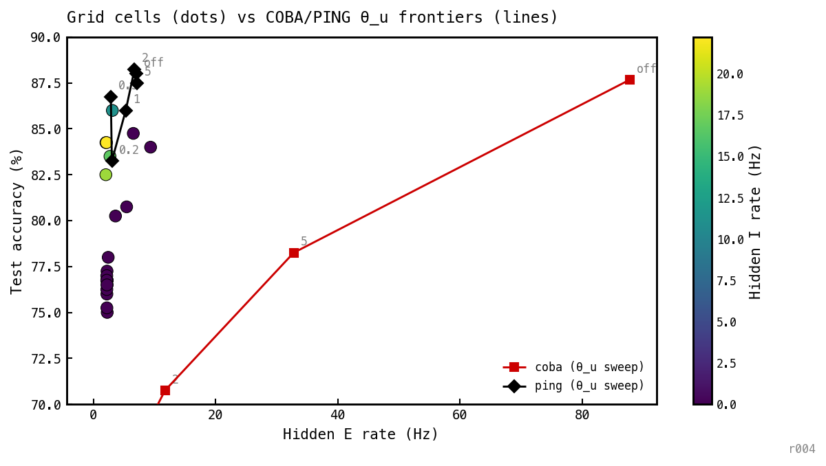
Grid scatter (coloured by I rate) plus the COBA (red squares) and PING (black diamonds) -sweep frontiers from nb025 Figure 5, connecting each model’s points. All curves and points trained for 100 epochs. Annotations on the frontier curves mark in spikes (or “off”). Note the axes follow the accuracy zoom (70–90%), so COBA’s low-rate tail at drops off the bottom.
The PING frontier sits above the green/yellow grid cluster — the -swept PING baseline reaches 85–89% accuracy at E rates 3–7 Hz, higher than the grid’s PING cluster (82–85.5%). This is because the canonical PING recipe uses but the grid was trained with (chosen to give no-loop cells a fair shot at converging), which costs a few accuracy points even at the recipe baseline coupling. The PING frontier also never leaves the active-loop regime even when the budget is squeezed all the way to 0.2 spikes — no value can push PING into the dark-purple band, because the loop sets a structural minimum on E rate. The grid scatter shows that the only way to reach that band is to start training from a init that prevents the loop from engaging in the first place — a structural rather than penalty-driven escape.
The COBA frontier sweeps across decades of E rate (≈88 Hz down to ≈0 Hz) at accuracies 88–62%. The interesting part is the low-E tail: at , COBA sits at — and the high-accuracy stretched-COBA grid cell at sits above this point at . So the grid solution is not just rediscovering COBA — it is finding a strictly better operating point than -squeezed COBA at the same rate, ≈10 pp higher accuracy with similar firing. This is the third attractor the diagonal slice also surfaces: not PING (no I loop), not penalty-squeezed COBA (different scale, different cell participation pattern), but a coupling-shaped E-only basin the optimiser only finds when initialised inside it.
Training videos
Per-epoch oscilloscope videos for every cell of the grid. Each video shows one epoch per frame against a fixed test trial; gamma cadence (if any) is visible in the E/I rasters. Naming: weiX__wieY for , .
| video | video | video | video | video | |
| video | video | video | video | video | |
| video | video | video | video | video | |
| video | video | video | video | video | |
| video | video | video | video | video |
1D diagonal slice along the ei_ratio = 2 line
The grid above varies and independently, but the codebase’s standard PING recipe ties them via with . Restricting to that line gives a finer-grained view: one knob () at 10 values, tracking at twice the value, three seeds per value, 100 training epochs. Accuracy is reported as the per-cell best epoch. Same recipe as the grid otherwise (, ).
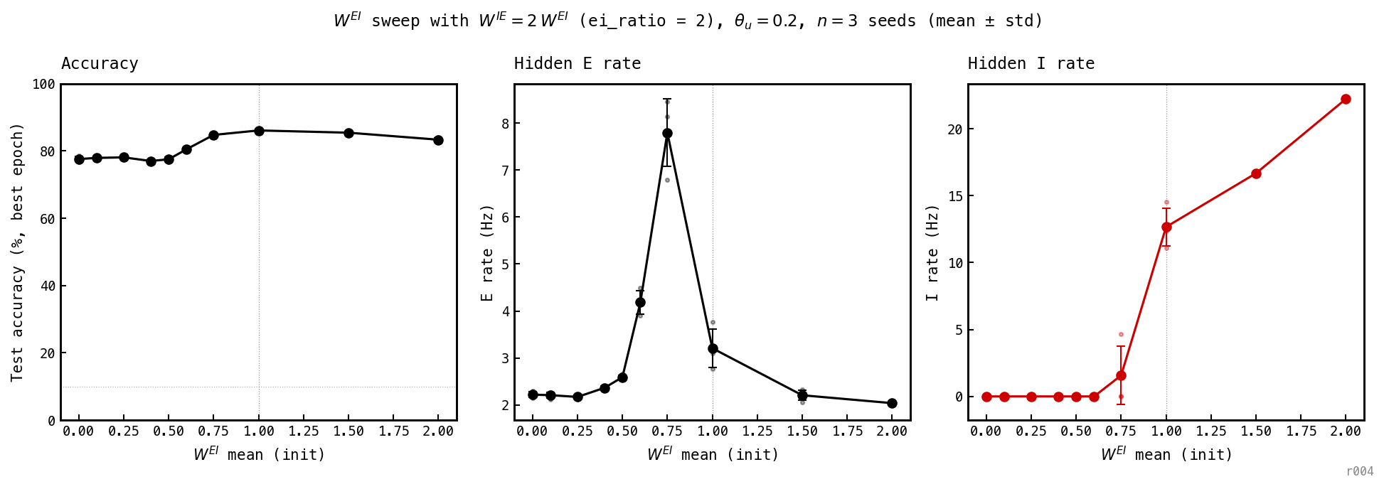
scanned over with . Error bars are mean ± std of the best-epoch test accuracy over 3 seeds (42, 43, 44), 100 training epochs each; faint dots show individual seed peaks. Left: test accuracy. Middle: hidden-E rate (last-epoch). Right: hidden-I rate (last-epoch). Grey dotted vertical at marks the canonical recipe baseline.
Three regimes:
- — no-loop / stretched-COBA, low-accuracy variant: accuracy 77–78%, I rate exactly 0, E rate 2.2–2.6 Hz. Tight error bars (acc std ≤ 0.9%) — the optimiser deterministically lands in the same E-only basin from any seed.
- — high-accuracy stretched-COBA, transition: 80.50 ± 0.43% accuracy, I rate still exactly 0 for all three seeds, E rate 4.18 Hz. The loop hasn’t engaged but accuracy is already 3 pp above the low-band.
- — transitional with weak loop: 84.75 ± 0.43% accuracy, I rate 1.6 Hz (1 of 3 seeds engages a small I population), E rate 7.80 Hz. The first cell on the sweep where I lifts off zero.
- — full PING: accuracy 85.4–86.1%, I rate climbing 12.7 → 16.7 Hz as the loop tightens, E rate clamped to 2.2–3.2 Hz by inhibitory negative feedback. The recipe baseline at is the peak of the sweep.
- — over-inhibited: 83.33 ± 0.63% accuracy, I rate 22.2 Hz, E rate 2.0 Hz. The drop from the plateau is ≈ 3 pp — not catastrophic, but the over-inhibited corner is genuinely less accurate.
The accuracy cliff is now smoother than the 30-epoch picture suggested. The accuracy cliff rises in two steps: (77.5% → 80.5%) and (80.5% → 84.75%). The I-recruitment cliff sits at the second step, between (I = 0) and (I ≈ 1.6 Hz). In the gap between the cliffs sits the high-E stretched-COBA solution at , which uses pure E firing without engaging the loop. With more compute the network finds an E-only solution that closes much of the gap with PING — the loop is a useful but not necessary mechanism for high accuracy at this spike budget.
Plotting the 30 cells in (E rate, accuracy) space — colour-coded by I rate, same convention as Figure 2b — makes the new attractor visible directly:
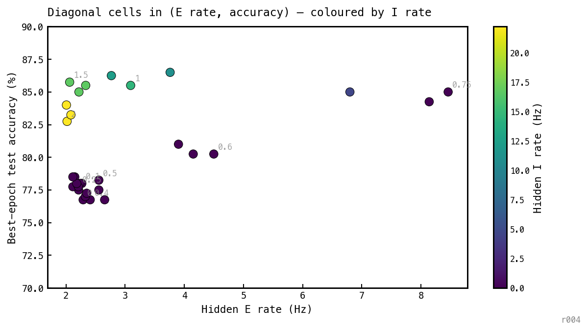
Each dot is one cell of the 100-epoch diagonal sweep, plotted at its best-epoch test accuracy vs final hidden-E rate. Colour encodes hidden-I rate; labels mark the value at one representative seed.
The diagonal scatter resolves the same physics as Figure 2b at higher resolution. The dark-purple () cluster now visibly splits into two sub-clouds: a low-E group (, E ≈ 2.4–3.7 Hz, acc ≈ 77%) and a tight knot at (E ≈ 7.7 Hz, acc ≈ 81%) — the high-accuracy stretched-COBA solution. They share the silent-I label but separate cleanly in . The green/yellow PING cluster () sits above at 82–85% accuracy with E rates clamped to 2–5 Hz by inhibitory feedback. The recruitment of inhibition (purple→green colour transition) and the accuracy cliff (vertical jump) happen at the same step in this slice (0.6 → 0.75), but the two purple sub-clouds prove that high accuracy is achievable on either side of the I-recruitment threshold — just at very different E rates.
Discussion
The map separates two accuracy basins — a high-E silent-I stretched-COBA solution and a low-E loop-engaged PING solution — that share the loss surface but live at very different per-spike economy. The PING corner is not uniquely optimal for accuracy at this tier, but it is the only corner where the E rate is held down to single digits; the rest of the per-spike-economy story in ar009 lives there.
Next steps
- Run the same diagonal at full MNIST + more epochs to check whether the two basins converge or stay separated.
- Sweep and independently (off-diagonal) to see whether the I-recruitment threshold tracks the product or one factor alone.