033 — Mean field model
Abstract
nb025 characterised the PING rate floor empirically: a recruitment cliff where the I-loop engages, gamma at ≈25 Hz. Both are bifurcation behaviours, and this entry pins them down in a mean-field model — with three goals and no more: locate the Hopf, predict its frequency, and classify it super- or subcritical. The right object is the 4D conductance mean-field : the Hopf is a linear fact about its Jacobian (giving Hz, in the spiking network’s gamma band and tracking its dependence on ), and direct simulation classifies it supercritical. The tempting 2D rate model cannot host the rhythm at all — provably, by Bendixson–Dulac, and because the reduction that produces it is not even asymptotically valid — so the analysis stays in 4D throughout.
Methods
Why a 2D model is the wrong object
The textbook tool for a bifurcation in an E/I circuit is a 2D Wilson-Cowan rate model: two population rates with sigmoid gains and instantaneous E↔I coupling. The PING architecture carries no recurrent E→E or I→I synapse (), so the model is
It is the wrong object, for two reasons.
The reduction isn’t valid. Collapsing the full conductance-based dynamics to (1) means adiabatically eliminating the synaptic conductances — legitimate only if they relax fast relative to the rhythm. They do not: – ms is the same order as the gamma period itself ( ms at 40 Hz). The inhibitory decay is not a slaved fast variable, it is the clock that sets the period. With no timescale separation to exploit, the elimination that produces (1) is unjustified — (1) is not a simplification of PING, it is a different system.
And even if you force it, it cannot oscillate. The divergence of the planar field (1) is pinned to a strictly negative constant,
because ‘s argument carries no and ‘s carries no — with no E→E or I→I synapse the gain multiplies only the off-diagonal cross-terms (it sets the rotation rate, never the divergence). By the Bendixson–Dulac theorem a planar flow whose divergence holds one sign on a simply connected region encloses no periodic orbit; so (1) sustains no limit cycle for any drive, coupling strength, gain shape, or amplitude — not merely no Hopf, but no oscillation anywhere in phase space. (The local face of the same fact: the Jacobian trace of (1) equals (2) everywhere, so it never reaches the a Hopf requires.) Consequently any 2D rate model that does oscillate has to import a destabiliser PING lacks — recurrent excitation in Wilson-Cowan, a cubic self-gain in FitzHugh-Nagumo — so it reproduces the rhythm through a fictional mechanism rather than approximating the real one.
What’s missing is the delay. What actually destabilises the silent state is the round-trip phase lag of the loop — E excites I after , I shunts E after — and (1), with instantaneous coupling, has discarded exactly it: inhibition that tracks with zero delay can only damp, never overshoot. Holding the lag is irreducibly more than two-dimensional — either keep the two synaptic conductances as first-order states (the 4D model below, whose synaptic poles rotate a complex pair across the imaginary axis at a Hopf), or write the delay explicitly (a delay-differential equation, whose transcendental characteristic quasi-polynomial carries infinitely many roots). So the analysis stays in 4D. “Local analysis near the Hopf” is done in the 4D coordinates — the Jacobian crossing below, and the amplitude law of §3.2 — never by swapping in a planar system.
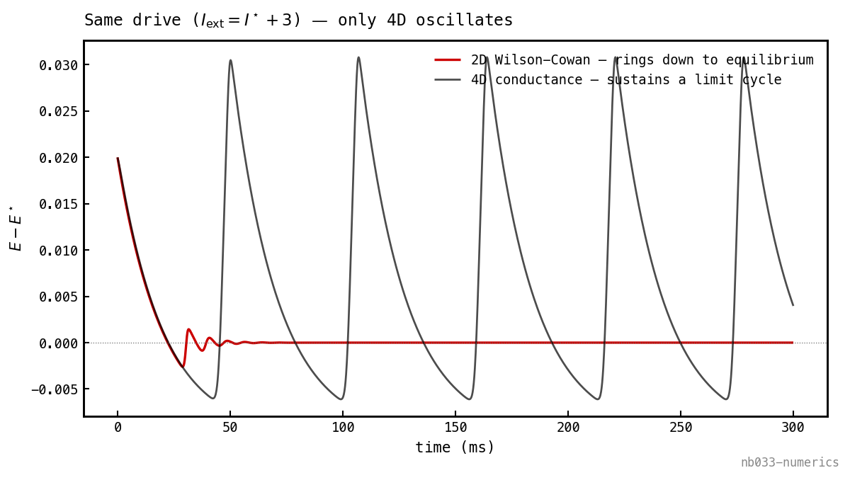
Bendixson made visible. Started from the same small kick at the same supra-threshold drive (), the 2D Wilson-Cowan field (1) (red) rings down to equilibrium, while the full 4D conductance model (black) settles into a sustained gamma cycle. The synaptic delay the 2D model eliminated is the entire difference.
The 4D mean-field model
We start with coupled conductance-based spiking neurons and reduce them, step by step, to four coupled ODEs for the population-mean rates and the population-mean conductances . Each step replaces one degree of freedom with a smoother, lower-dimensional approximation; the cost of each is recorded at the end. The full chain is:
-cell spiking COBA → homogeneous-coupling spike-train integrals → population-mean rates and conductances → driving-force linearisation → relaxational rate dynamics with f-I gain → final 4D system in .
Step 1. Single-cell COBA equations. Index E cells by and I cells by . From the methods paper ar009 eq. (1) with the architecture constraints (no recurrent E→E, no I→I) and an external drive added on E:
The E cell has no term because the only excitation it receives in this analysis is (the feedforward drive); the I cell has no because there is no I→I coupling. The conductances are themselves driven by presynaptic spikes through first-order linear filters:
with the spike train of E-cell as a sum of Dirac pulses at its firing times (similarly for ). (D2a–b) are the continuous-time forms of eq. (8) and (7) in the methods backbone — exponential synapses with per-spike weight and decay .
Step 2. Homogeneous coupling. The weight matrices in the simulator are random with finite variance. Replace each entry by its population mean: and for all . The presynaptic-summation terms in (D2a–b) become
where we introduce the population-mean firing rates
Strictly, and as defined are sums of deltas. The mean-field interpretation is that under a smooth-rate ansatz — averaging over a short window or assuming a continuous spiking density — we treat as smooth functions, so becomes an ordinary continuous source term. (D3) drops two things: weight heterogeneity, and finite-size fluctuations. The latter is the stochastic noise that survives in any actual finite population: even with all weights at their mean values, the population rate is a sum of independent point-process samples, so it has shot-noise variance over a short window. The mean-field limit takes at fixed , in which the law of large numbers makes converge to their expected values and the variance vanishes. At finite the residual fluctuations act as a noise term on (D4), which (a) smears the Hopf bifurcation — instead of a sharp onset, the spiking simulator shows a rounded shoulder with sub-threshold variance — and (b) maintains a low-amplitude noisy gamma oscillation just below criticality where the linearised mean-field predicts strict silence. Both effects reappear in the spiking simulations, with magnitude controlled by .
Because the source terms (D3a) and (D3b) no longer carry a cell index, every E cell sees the same and every I cell sees the same . The per-cell conductance equations collapse to two population-mean equations. Defining lumped couplings
(carries-the-fan-in: each E spike contributes the per-edge weight, and there are presynaptic E cells), the conductance dynamics become
Two equations down from . (Note: the absolute scale of folds into used in the final 4D system after Step 5.)
Step 3. Driving-force linearisation. The synaptic terms in (D1) still depend on through factors and . Take to its resting value in the synaptic terms only (not in the leak or the threshold-crossing, which we’ll handle separately via the f-I curve). With mV and the reversal potentials from ar009,
(so mV — depolarising drive on I). The synaptic currents in (D1a–b) become
— each synaptic input is now linear in conductance, with the cell-population-independent prefactor folded into a constant. This is the crucial reduction: it kills the multiplicative coupling between membrane potential and synaptic conductance that makes COBA so different from CUBA, but only in the driving force. Shunting (the effect of on and ) is dropped at this step; this is what the table at the end records.
Step 4. Population rate from an f-I curve. Under (D5) the membrane equations (D1a–b) have the form — exactly LIF with a synaptic current. A LIF cell receiving constant net input current fires at rate where is its f-I curve. Replacing each cell’s spike output by its rate response gives
with effective input currents (from D1 with D5 substituted)
(I cells receive only excitation in this architecture; E cells receive external drive minus the GABA shunt.) The instantaneous-rate replacement (D6a) is only valid when input changes are slow compared to the membrane integration time. In reality, relaxes toward the f-I-curve fixed point on its membrane time constant . Encode this with an explicit relaxation:
where are the smooth steady-state gain functions (sigmoids in the numerics). Drives that change faster than are filtered; the rate doesn’t snap to the f-I curve instantaneously. Two more equations down — together with (D4a–b) we now have four equations in .
Step 5. Absorb the driving-force constants. The fixed prefactors in (D7) and the fan-in scalings in (D4) are just multiplicative constants — they don’t carry dynamical information. Fold them into the couplings:
and likewise absorb the inside the I-cell argument by redefining (similarly for ). The conductances now have units of input current rather than µS; the f-I curves take their argument directly. This change of variables is pure bookkeeping — no dynamics are lost.
The four equations after (D4) + (D7) + (D8) are exactly the 4D system shown next.
| Step | Approximation | What’s lost |
|---|---|---|
| D3 | homogeneous coupling, smooth-rate density | weight heterogeneity, finite-size noise |
| D5 | in driving force | shunting, threshold-crossing nonlinearity |
| D7 | single relaxational mode at | sub-membrane dynamics, refractoriness |
| D8 | absorb constants into and | nothing (bookkeeping only) |
The 4D system
After Steps 1–5, the mean-field equations are
in state . Whether this 4D state is minimal — or a 2D reduction would do — was settled in Why 2D reductions fail: the synaptic phase delays are load-bearing, and a planar model that eliminates them cannot oscillate. The 4D state keeps them.
4D Jacobian
At a fixed point :
with evaluated at the fixed-point arguments.
Results
Of the three goals, two are linear — locating the Hopf and reading off its frequency are facts about the Jacobian — and one is nonlinear — whether the bifurcation is super- or subcritical. We take them in that order.
Frequency
We locate the bifurcation numerically: sweep , track the fixed point (near-silent until the loop engages), and diagonalise at each step. The recruitment cliff is a Hopf bifurcation — the smallest at which a complex-conjugate eigenvalue pair reaches the imaginary axis (, ), so the silent fixed point loses stability to a growing oscillation rather than to a static shift. The crossing frequency is the gamma frequency, .
For the canonical parameters (, , , ms; , ):
That Hz sits squarely in the PING gamma band. It is not a parameter-free number — the mean-field’s abstract coupling units set the overall scale — but the dependence on the synaptic timescales is the predictive content, and across a sweep it tracks the spiking network’s gamma (Figure 3 below).
Tracking all four eigenvalues does double duty. At onset exactly one complex pair reaches the imaginary axis while the other modes stay well damped, so this is a simple, generic Hopf — not a double-Hopf where two pairs cross together (which would spawn tori the linear frequency cannot capture). That is precisely the condition under which a local near-onset analysis is valid. The complex plane shows the crossing and reads off the frequency at once:
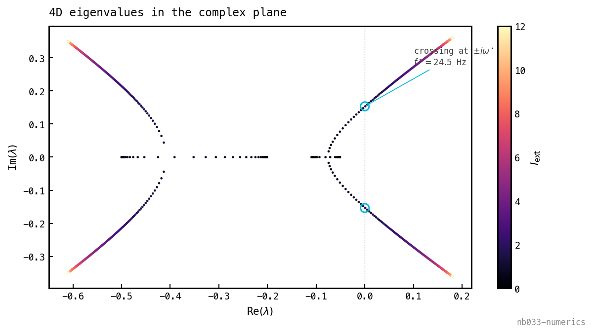
The four eigenvalues as sweeps (colour = drive). One conjugate pair marches right and crosses the imaginary axis at (cyan circles) at , reading off Hz directly as the crossing height; at onset the other modes sit safely in the left half-plane — the simple-Hopf certificate, seen geometrically. (A second pair only reaches the axis at far higher drive, well above the recruitment cliff.)
Does the frequency track the synaptic clock? The mechanistic claim is that sets the period. Re-finding the Hopf at each in nb041’s retrained sweep and overlaying the spiking network’s measured :
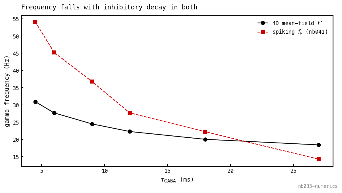
Both fall monotonically with — the inhibitory decay is the clock in both. The match is qualitative, not quantitative: the mean-field is flatter, under-predicting at short (24.5 vs 37 Hz at 9 ms) and slightly over-predicting at long , with the curves crossing near 20 ms. The reduction captures the mechanism but not the full sensitivity — expected, since it drops the spike-synchrony of the E-volley that sharpens the cycle most at short .
Which coupling moves the cliff? Sweeping the recruitment threshold across the plane recovers nb025’s empirical asymmetry from the equations:
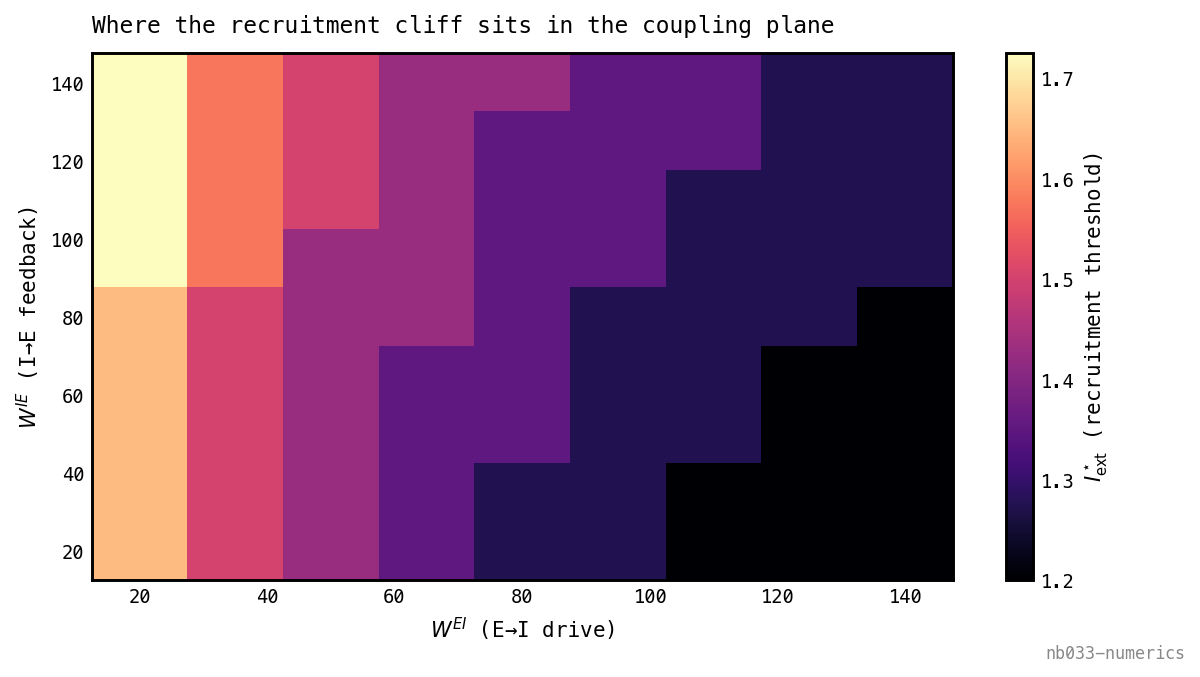
The Hopf threshold over the coupling plane. It varies more strongly along (E→I drive) than along (I→E feedback): the mean-field makes the dominant knob on the recruitment cliff — consistent with nb025’s ” moves the cliff” — with only a weak secondary dependence (the faint diagonal). Ties to nb036’s coupling-plane basins.
Super or subcritical
The eigenvalue crossing says a limit cycle is born at but not whether it appears with zero amplitude (supercritical, soft onset) or with a finite jump and hysteresis (subcritical, hard onset). That is a nonlinear question, classically the sign of the first Lyapunov coefficient of the Hopf normal form. We read it off the full 4D field by direct simulation instead: integrate (3)–(4) from a small perturbation of the fixed point across a grid of straddling and measure the steady-state peak-to-peak amplitude — the full top-to-bottom swing of the population rate once settled, , which is exactly zero at a fixed point and positive the instant a limit cycle exists (no period-fitting or cycle-centre needed, the appeal of the direct measure). This needs no center-manifold reduction and no assumption that the local picture is 2D — and it is self-checking, since a hidden degeneracy would show up as beating or quasiperiodicity in the amplitude trace rather than the clean law below. Below the perturbation decays to zero; above it the amplitude grows continuously from zero, with (linear fit slope , ). The square-root amplitude law and the absence of any jump or hysteresis mark a supercritical Hopf — the network slides smoothly from silence into a small-amplitude gamma cycle as drive crosses threshold, exactly the soft recruitment cliff of nb025.
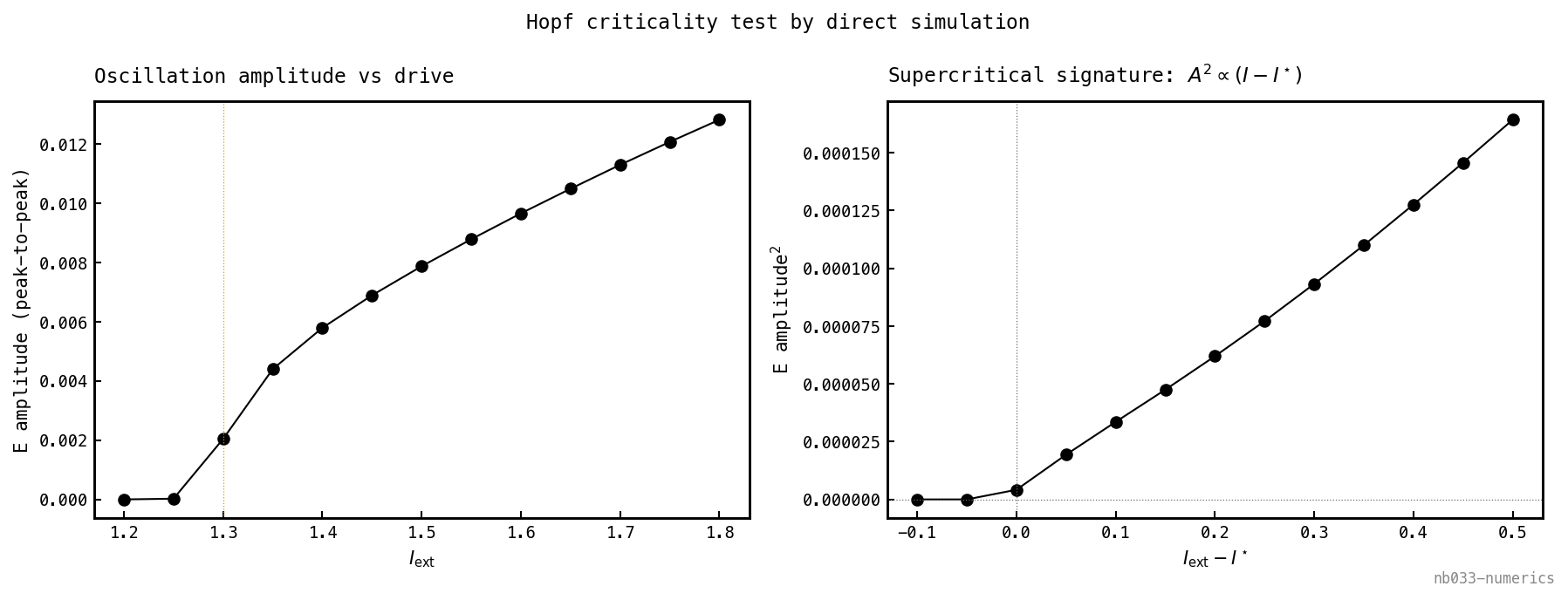
Amplitude is zero below and grows continuously above it (left); is linear in (right, slope , ). No jump, no hysteresis — a soft onset.
Why that shape is supercriticality. The square-root law is not a fit — it is forced by the Hopf normal form, which is what lets the measured curve stand in for the Lyapunov coefficient we declined to compute. Near the crossing the oscillation amplitude obeys a radial flow , with the growth rate of the now-unstable pair and the first Lyapunov coefficient. The limit cycle is the balance , i.e. : a stabilising cubic () gives a real cycle of radius — the linear instability pushes the amplitude out, the cubic reins it in, and they settle at a small finite radius. So ” linear in ” is equivalent to , which is the definition of supercritical; a subcritical Hopf () has a destabilising cubic, no small stable cycle, and an amplitude that appears with a jump and hysteresis — neither in the sweep. (It is the dynamical twin of a second-order phase transition: the gamma amplitude is the order parameter and the exponent the mean-field critical exponent.)
The slope carries one more reading. Since , the sensitivity diverges at threshold: the amplitude rises with a vertical tangent, so the rhythm switches on smoothly (no jump) yet steeply — most of its amplitude appears in a thin sliver of drive just past . Soft, but sharp: the dynamical content of nb025’s recruitment cliff.
The cycle the onset produces, just above threshold:
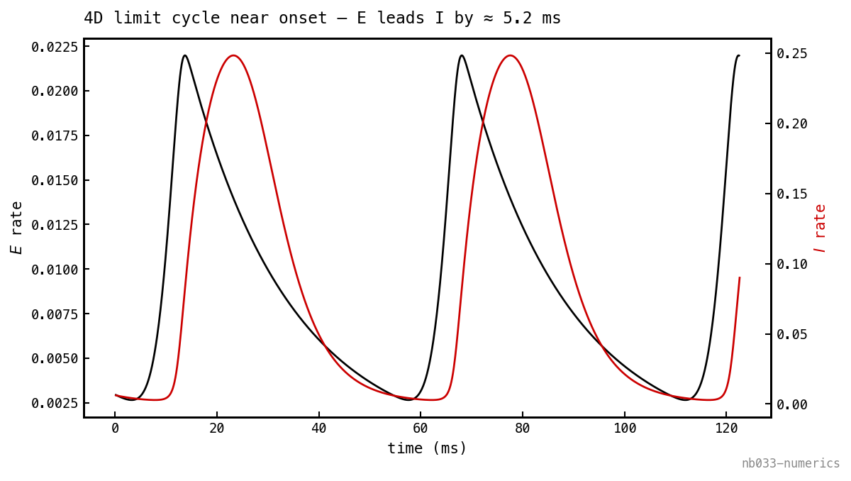
(black) and (red) over the limit cycle at . The E burst leads the I burst by ≈ 5 ms — the loop delay made visible: E recruits I, I shunts E a few milliseconds later, and the cycle turns over. This is the round-trip phase lag the 2D reduction throws away.
Discussion
The 4D Hopf (Figure 2) locates the recruitment threshold and a gamma frequency Hz from the synaptic timescales and coupling matrices — in the spiking band, reproducing its -dependence (Figure 3) and nb025’s ” moves the cliff” asymmetry (Figure 4), though flatter in absolute Hz than the spiking network. The 2D reduction shows why the full 4D state is needed: with it cannot destabilise the silent fixed point (Bendixson–Dulac, Figure 1), because the oscillation is driven by the synaptic phase delays the reduction throws away. The mean-field thus pins the mechanism of the factor in nb041’s affine law (the per-cycle participation being the separate, spike-resolved result of nb046); the quantitative frequency calibration is approximate and left to the spiking network.
A note on the “use a 2D model” instinct, since it is the natural one: it is right about the analysis and wrong about the object. All three results here are local near the Hopf — the Jacobian crossing, the frequency, the amplitude scaling — and a Hopf is generically a 2D phenomenon. But the legitimate 2D-ness is the center-manifold normal form derived from the 4D field, not a Wilson-Cowan or FitzHugh-Nagumo system substituted for it. The appendix carries out exactly that reduction — Kuznetsov’s first Lyapunov coefficient computed from the 4D Jacobian and gain derivatives — and it agrees with the direct simulation on the sign (), the frequency, and the amplitude slope to ≈ 4%. Working in 4D coordinates throughout keeps the local analysis honest and keeps the parameters mapped onto things the circuit actually has (, ) rather than onto a fictional recovery variable. “Reduce locally for the analysis, keep 4D as the object” is one position, not two.
Appendix — the normal form, derived from the 4D field
§3.2 settled super- vs subcriticality by simulation, with no theory required. This appendix does it the textbook way as well — the first Lyapunov coefficient — and checks the two agree. It also makes concrete what “go locally 2D near the Hopf” actually means, since that phrase is easy to misread.
The idea, in words. Near the Hopf the 4D system has four modes (eigen-directions of the Jacobian): one oscillating pair, barely stable, that is about to become the gamma rhythm, and two others that decay fast. “Fast” relative to the barely-stable gamma mode means that whatever state you start in, those two collapse almost immediately, and the long-run behaviour — the limit cycle and whether it switches on softly or with a jump — plays out on a 2D surface carrying the gamma mode. That surface is the center manifold; the equation for the dynamics on it is the normal form. So near onset the essential dynamics genuinely are 2D.
Two things to keep straight, because they are exactly where the “2D” word causes trouble:
- Those 2D coordinates are not the rates . They are the amplitude and phase of the gamma mode — a direction that mixes all four variables.
- This is therefore not the Wilson-Cowan / FitzHugh-Nagumo rate model §2.1 rejected. That model eliminates the conductances (wrong — they carry the delay); the center manifold keeps the full 4D field and merely drops the directions that decay fast, so the delay — hence the frequency — stays in. The center manifold is the legitimate “go 2D,” derived from the 4D field rather than substituted for it.
What we need. Three things, all read off the 4D Jacobian at the Hopf:
- the frequency — the imaginary part of the critical (purely imaginary) eigenvalue, ;
- the critical eigenvectors and : points along the gamma mode (), and is its dual partner (, normalised so ), used to measure “how much gamma mode” a given state contains;
- how the field’s curvature — its quadratic and cubic terms — bends the gamma mode back on itself.
On the center manifold the dynamics become , where is the complex gamma amplitude, is the growth rate past threshold, and is the cubic term that saturates it. One number decides everything, : negative, the cubic pushes back → supercritical (soft onset); positive, it pushes out → subcritical (hard onset). This is the same balance behind §3.2’s square-root law — is just its sign, computed rather than measured.
The curvature is almost all zero. The only nonlinear parts of the 4D field (3)–(4) are the two gain curves: the E-equation bends through , the I-equation through , and the conductance equations are perfectly straight lines. So the quadratic form (the second derivatives) and cubic form (the third derivatives) each have a single non-zero slot — with state order ,
with (the gain’s curvature) and (its rate of change of curvature) evaluated at each gain’s fixed-point drive — for E, for I.
The formula. Feeding these into Kuznetsov’s projection formula — the standard recipe for reading off a vector field of any dimension (Elements of Applied Bifurcation Theory, eq. 10.59):
It looks forbidding but it is pure bookkeeping: project the cubic curvature onto the gamma mode, then subtract the two ways the quadratic curvature feeds back through the off-mode directions (the matrix solves and route those quadratic “overtones” back onto the mode), and take the real part. Two linear solves and three dot products, evaluated once at the fixed point.
The result. Refining the Hopf to where the pair is exactly imaginary (, rad/ms, i.e. Hz — matching the sweep’s 24.5 Hz) and evaluating:
Negative, so the analytic verdict is supercritical — exactly §3.2’s, now with the center-manifold-validity assumption made explicit rather than implicit (the “only one mode crosses” condition that licenses the whole reduction was certified back in Figure 2).
Does it match the simulation? Quantitatively. The normal form predicts more than a sign. The cycle radius is , and at leading order the measured peak-to-peak E amplitude is (with the E-component of the gamma mode ), so
With and the eigenvector, this predicts an onset slope of — against the measured by direct simulation (Figure 5): a ≈ 4% match. The small gap is leading-order truncation — the simulation runs at finite amplitude out to , where the higher-order () terms the normal form drops start to matter.
The verdict. Sign, frequency, and amplitude slope all agree between the analytic normal form and the direct 4D simulation. So “go locally 2D near the Hopf” is real and legitimate here — and it is this center-manifold reduction of the 4D field (its eigenvectors , its curvature forms ), not the rate model §2.1 ruled out.