024 — Training
Abstract
Training recipe (canonical / medium tier):
| Parameter | Value |
|---|---|
| Integration timestep | 0.1 ms |
| Trial duration | 200 ms |
| MNIST samples (80/20 stratified split of 2000) | 1600 train / 400 test ( 2.9% of the 70k-sample MNIST corpus) |
| Epochs | 100 |
The convergence diagnostics in nb041 and nb044 showed the same pattern: test accuracy plateaus within ~ 10–15 epochs while the trained E rate keeps drifting upward through epoch 30. This entry asks the simple follow-on question — does the rate stabilise if we let training continue, and if not, why not?
Methods
Train PING and COBA (loop disabled, = off) from scratch for 100 epochs instead of nb025’s 30. Three seeds per architecture (42, 43, 44) = six cells total. Medium tier sample count (2000 training samples, 400 test). All other PING / COBA recipe parameters held to nb025 — same Adam at , mem-mean readout, no rate regulariser.
Per-epoch metrics captured: test accuracy, CE loss (train + test), mean E and I firing rate, activity fraction (what fraction of cells fire at all), gradient norm, and per-parameter Frobenius norms of every trainable weight (a small addition to the trainer for this audit). After training, additionally run inference on the final weights to recover per-cell firing-rate distributions.
The slope across the last 10 epochs on each metric is the operational definition of “converged” — values below 0.1 pp/ep (accuracy) and 0.05 Hz/ep (rate) per cell.
Results
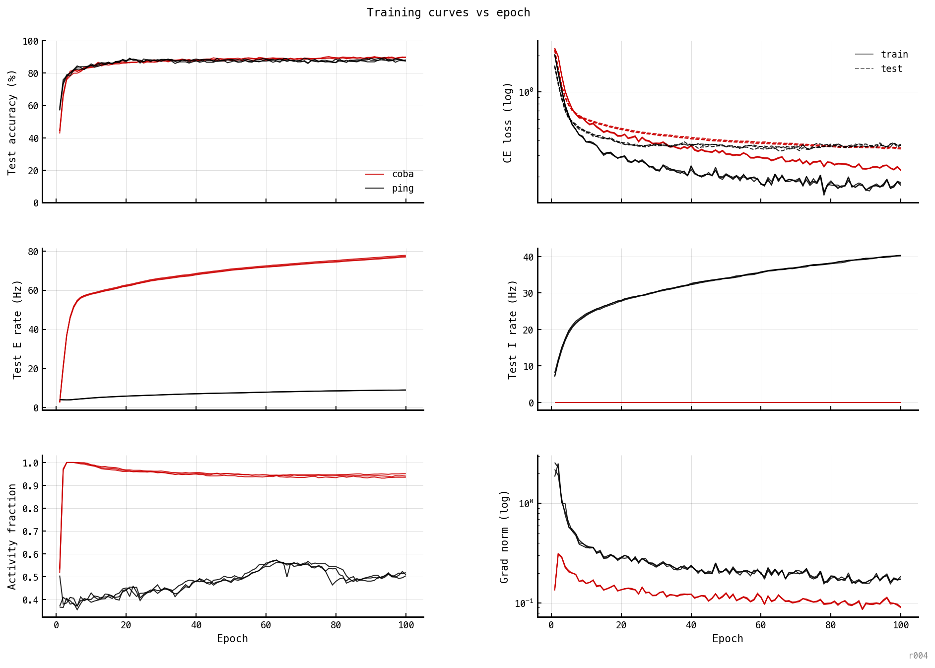
Six per-epoch metrics for PING (black) and COBA (red), three seeds each. Accuracy and loss converge by epoch ~ 15 in both architectures; E rate is the slow-changing variable.
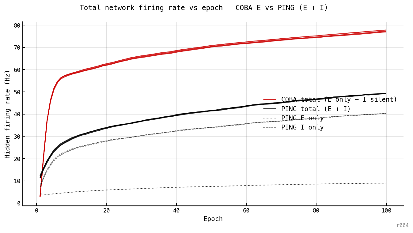
Honest like-for-like comparison of the total spike budget each architecture spends. COBA’s I population is silent (ei_strength = 0 → no recurrent input to I), so its hidden-network total is just its E rate. PING’s total is E + I summed. The headline 10× E-rate gap shrinks to ≈ 1.6× when total network spikes are counted (PING ≈ 49 Hz vs COBA ≈ 77 Hz at epoch 100). The decomposition: PING’s E rate (dotted) is the locked variable that sits at 4–9 Hz throughout — the gamma cycle’s per-cell participation ceiling — while PING’s I rate (dashed) tracks the same climbing trajectory as COBA’s E rate, both driven by the still-growing . The architectural gating is specifically on E; the I population fires nearly as hard as COBA’s E does. (Note: population sizes are and ; a population-weighted per-cell total would give COBA Hz and PING Hz — a 4× gap, intermediate between the 10× E-only and 1.6× E+I numbers.)
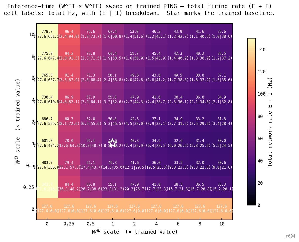
Inference-time sweep on the trained PING baseline (seed 42, θ_u = off, 100 epochs). For each cell of a 9 × 9 grid spanning multipliers 0 to 10, the trained and matrices are multiplied by the column / row scale factors before running the test set. Cell colour and large number: total network firing rate (E + I). Small numbers in parentheses: per-population (E | I) breakdown. White star marks the trained baseline at (1, 1). Three structural readings:
- Open the I→E direction (left column, ). E fires at 127.6 Hz everywhere (no inhibition ever reaches E). I is driven harder as grows (216 → 651 Hz) but does no inhibitory work. The loop is broken on this side.
- Open the E→I direction (bottom row, ). I never fires (silent at 0 Hz across the row). E runs free at 127.6 Hz. The loop is broken on this side too.
- The loop must be closed on both sides to engage. Once it is, total rate falls fast — and then asymptotes around 38–40 Hz across most of the engaged region. Pushing or to 10× the trained value doesn’t compress total rate below ~ 40 Hz; what it does instead is push the (E | I) split further toward I-dominated (e.g. at (10, 10), E ≈ 1 Hz, I ≈ 39 Hz). Strengthening compresses E within the loop; strengthening moves the recruitment cliff to lower input but doesn’t change the engaged-state rate much. This matches the inference-time asymmetry from nb036: controls whether the loop engages, controls how hard it compresses once engaged.
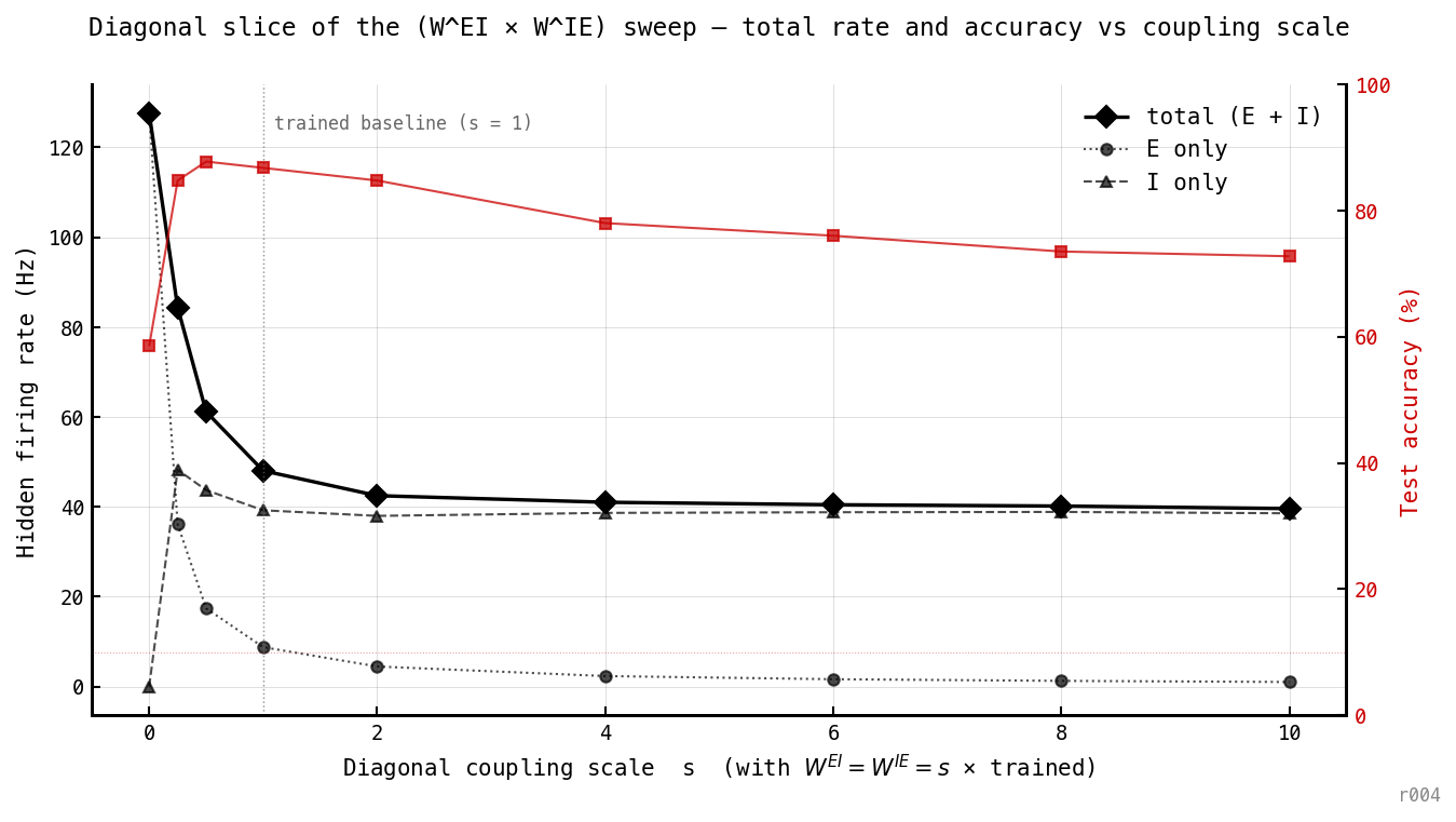
Bottom-left → top-right diagonal of Figure 3, redrawn as a line chart. As both edges of the loop strengthen together, total rate drops sharply through s = 0.25–1 and then asymptotes around 39–40 Hz by s ≈ 4. The compression bottoms out — there is no further win from pushing coupling beyond the trained baseline.
Three things to note:
- Accuracy peaks at s = 0.5 (87.75%) — slightly above the trained baseline at s = 1 (86.75%). The trained operating point is not the accuracy peak along this slice. The optimiser landed close to it (the gap is small) but the small mismatch is real and worth flagging — the rate regulariser may have pulled the recipe one notch past the accuracy peak.
- Beyond s ≈ 2, accuracy starts declining while total rate barely moves. Over-coupling buys nothing and costs classification.
- The asymptote is set by I, not by E. Past s ≈ 2, E rate falls to < 5 Hz and keeps declining toward zero, while I rate plateaus at ~ 38 Hz. The 40 Hz floor is essentially the I-population firing once per gamma cycle at Hz, regardless of how hard drives it or how aggressively suppresses E. The architecture has a total spike floor that can’t be moved below the I-cycle rate by coupling strength alone.
| Cell | Final acc | Final E rate | E rate slope (last 10 ep) | Acc slope (last 10 ep) |
|---|---|---|---|---|
| PING seed 42 | 87.50% | 9.01 Hz | +0.019 Hz/ep | −0.056 pp/ep |
| PING seed 43 | 88.25% | 9.05 Hz | +0.025 Hz/ep | +0.139 pp/ep |
| PING seed 44 | 87.50% | 8.95 Hz | +0.018 Hz/ep | −0.111 pp/ep |
| COBA seed 42 | 89.75% | 77.29 Hz | +0.135 Hz/ep | +0.028 pp/ep |
| COBA seed 43 | 90.00% | 76.93 Hz | +0.128 Hz/ep | −0.028 pp/ep |
| COBA seed 44 | 89.75% | 77.78 Hz | +0.125 Hz/ep | +0.000 pp/ep |
Two clean findings on convergence:
- PING’s E rate is a converged operating point. All three seeds land within 0.1 Hz of each other at Hz with slopes below 0.025 Hz/ep — a 50× margin below the strict 0.05 Hz/ep convergence threshold. The cross-seed reproducibility (8.95, 9.01, 9.05) is striking.
- COBA’s E rate has not converged. Slopes are 0.13 Hz/ep — 5× PING’s slope, above the convergence threshold. With another 100 epochs COBA would gain another ~13 Hz on top of the current ~77 Hz. The 30-epoch number from nb025 (≈ 88 Hz) and the 100-epoch number here (≈ 77 Hz) are both training-snapshots, not stable points.
Why is PING’s rate stable while COBA’s drifts?
The figure below shows two quantities per trainable parameter, per epoch. Definitions:
- — the input projection matrix ( for MNIST), the only trainable parameter mapping the Poisson-encoded image into the hidden E population.
- — the readout matrix (), the only trainable parameter mapping hidden E activity to logits.
- — the Frobenius norm of a weight matrix, . A single scalar magnitude per parameter that grows when the optimiser pushes weights away from the origin. A growing means the weights are still actively being adapted; a flat one means they have stopped moving.
- ratio — the mean per-step ratio averaged over the epoch. A scale-free measure of how strongly the optimiser is pushing each parameter relative to its current size. Values near mean active learning; means slow drift; and below means effectively frozen.
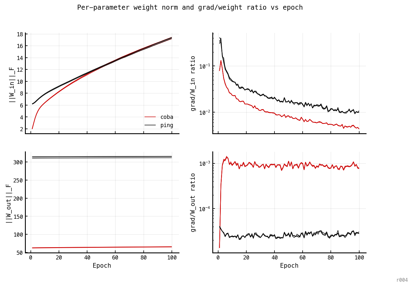
Top: ||W_in||_F (left) and grad/||W_in|| ratio (right). Bottom: ||W_out||_F (left) and grad/||W_out|| ratio (right). Both architectures’ W_in is still actively adapting; both architectures’ W_out is essentially frozen from epoch 1.
The rate drift is W_in’s work, not W_out’s. ||W_out||_F changes by 0.4% over 100 epochs for PING and 4.6% for COBA — both essentially frozen. ||W_in||_F grows 2.8× for PING and 8.8× for COBA, and is still rising at epoch 100. The naive “larger W_out pushes more spikes through the readout → higher rate” hypothesis is dead; the rate dynamics are entirely a story about input-weight adaptation.
PING’s grad/W_in ratio sits higher than COBA’s throughout training (top-right panel) — PING’s W_in is moving more aggressively per epoch — yet PING’s rate barely changes (0.02 Hz/ep) while COBA’s drifts (0.13 Hz/ep). So PING’s W_in adaptation produces useful classification gains without rate scaling, while COBA’s W_in adaptation is coupled to rate climb. The I-loop decouples weight adaptation from rate output.
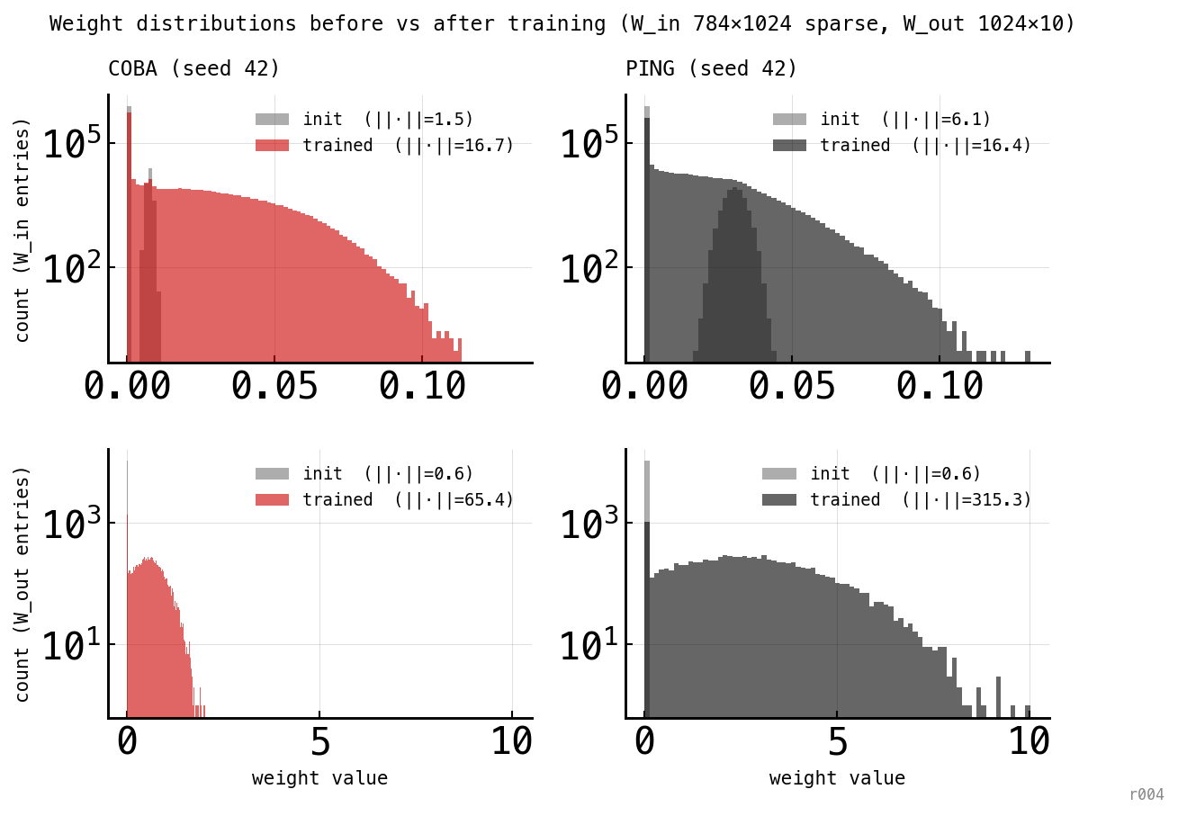
Histograms of every weight value, before training (grey) and after training (red for COBA, black for PING). Top row: W_in. Bottom row: W_out. Y-axis logarithmic. The Frobenius norm of each distribution is annotated in the legend.
The histograms make Figure 2’s norms concrete. W_in starts as a sparse near-zero matrix (95% of entries exactly zero per the —w-in-sparsity 0.95 recipe; the remaining 5% drawn from a narrow distribution); training spreads the non-zero tail into a long heavy distribution reaching ≈ 0.10 in both architectures. W_out is the more striking comparison: both start tightly clustered near zero, but the trained distributions look very different. COBA’s W_out is compact (max ≈ 2, ||·|| = 65). PING’s W_out is five times broader (max ≈ 10, ||·|| = 315) — because PING fires ≈ 10× more sparsely than COBA, its readout has to weight each surviving spike ≈ 10× more strongly to reach the same logit magnitudes. The readout adapts its scale to compensate for the rate gap; the rate gap itself is not visible in the per-weight value at the time-mean level.
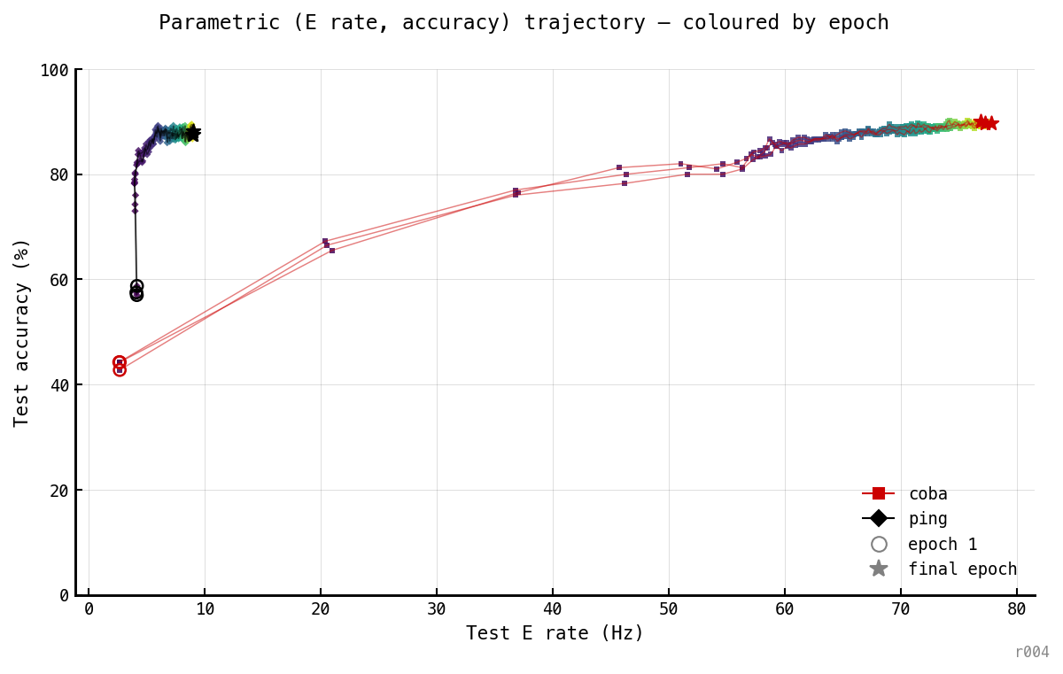
Test accuracy vs test E rate, one parametric curve per cell, epochs encoded as dot colour (epoch 1 = dark, epoch 100 = bright). Open circles mark epoch 1; stars mark final epoch.
The trajectory plot makes the architectural difference visible in one figure. PING walks straight up the y-axis (single attractor at ~9 Hz); COBA walks diagonally and then traverses along the high-accuracy plateau — the rate keeps climbing at constant 88–90% accuracy. PING has a single attractor; COBA has a manifold of equally-accurate solutions parameterised by rate, and gradient descent drifts along it.
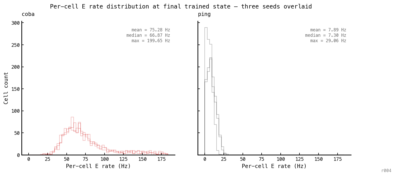
Per-cell E firing rate histogram at the final trained state. Left: COBA. Right: PING. Three seeds overlaid per panel.
The rate distribution shape is qualitatively different between architectures, not just shifted. PING has a narrow distribution capped at ~30 Hz with ~9% of cells silent. COBA has a long heavy right tail with cells firing at 200 Hz. The architectural ceiling shows up at the per-cell level, not just the population mean — no individual E cell in PING fires above 30 Hz, regardless of which seed.
Discussion
The 100-epoch audit settles two questions for ar010:
- PING’s ≈ 7-9 Hz rate floor is a converged operating point. The paper can cite the rate as a converged value rather than a training-snapshot. The cross-seed consistency at 0.1 Hz precision is itself a strong claim — the gamma rhythm pins the rate to a tight tolerance independent of initialisation.
- COBA’s rate is open-ended. The 88 Hz number from nb025 (30 epochs) and the 77 Hz number here (100 epochs) are both in-training snapshots. The paper should present COBA’s rate as “drifting in the high-rate manifold” rather than as a fixed comparator. The order-of-magnitude separation between the architectures is what’s robust; the specific COBA number is not.
The mechanism diagnostic from the weight-dynamics figure also clarifies what the I-loop is actually doing in the trained network: it decouples input-weight adaptation from rate output. PING continues to adapt W_in throughout training, gaining classification accuracy without the rate climbing — the gamma cycle gates the spikes per cycle to a fixed budget regardless of the underlying drive. COBA has no such decoupling, so any W_in growth feeds straight through to higher firing.
The trajectory plot offers a geometric framing of the trained-network reachable sets: PING’s training trajectory sits in a point attractor in (rate, accuracy) space; COBA’s sits on a manifold. Under any gradient pressure that pulls rate away from PING’s attractor, accuracy is paid; COBA can drift along its manifold without paying.
Next steps
The collection’s headline rate numbers were measured at 30 epochs of medium-tier training. nb024 shows that PING converges at that horizon but COBA does not, and that W_in continues to adapt past epoch 30 in both architectures. Concrete follow-ups per notebook in the collection:
- nb033 — Mean-field PING. The 4D Hopf predicts Hz. Predict the rate from using parameters derived analytically from the mean-field gain functions and compare to nb024’s converged 9 Hz. A match would close the theory ↔ trained-network loop quantitatively.
- nb025 — Why PING has a rate floor. The headline empirical entry. Re-run at 100 epochs. The PING ≈ 7 Hz baseline becomes PING ≈ 9 Hz (converged); the COBA ≈ 88 Hz number becomes ≈ 77 Hz (still drifting but closer to its long-run attractor). The 13× E-rate gap claim becomes a 9× E-rate gap at converged values. Honest total (E + I) rate gap at convergence is ≈ 1.6× — see Figure 2 above. The structural claim that survives both definitions is the per-cycle E-participation gate, not a global power reduction.
- nb036 — Which E↔I weights set the recruitment threshold. The scaling fit is a cliff position, not an absolute rate, so it should be insulated from the convergence issue. Worth re-checking the 5×5 training-grid figure at 100 epochs to see whether the PING / stretched-COBA / no-loop cluster boundaries shift.
- nb037 — Dropping and adding spikes in trained PING. Inference-only on the trained baselines. The drop / add perturbation curves and the inference-only sweep should be re-run on the 100-epoch nb025 weights once those exist. The qualitative result (drop preserves cycle; add corrupts it) should survive; the specific numbers will tighten.
- nb038 — f-I curves and inference-time loop transfer. Inference-only. Re-run on 100-epoch nb025 baselines. The recruitment cliff position in input-rate space is the load-bearing finding and should be invariant.
- nb041 — Rate floor tracks gamma frequency (retrained). Re-run at 100 epochs. This is the highest-priority re-run after nb025. The affine fit at 30 epochs gave Hz, , . At 100 epochs the slope will shift upward (PING rates climb modestly) and the cross-seed variance will tighten. The should not move. The structural-bound argument is robust; the specific coefficient cited in ar010 should anchor at the converged value.
- nb042 — Rhythm vs mean-inhibition. Inference-only on nb025 weights. The 3.2× phase-shuffle release was measured against the 30-epoch baseline. Re-run against 100-epoch baselines; the multiplier should be similar (the mechanism is conductance arithmetic, not training duration) but worth confirming.
- nb044 — Δt audit. Re-run at 100 epochs for the coarse-Δt cells where the rate was still rising fastest. The cycle-period-Δt-invariance finding is robust because it’s a dynamic-system property; the rate-vs-Δt scaling slope is the part that needs converged values.
- nb024 — this entry. No follow-up needed for the convergence question itself. The geometric framing of the (rate, accuracy) trajectory plot is the most generalisable finding and deserves to be lifted into ar010’s Discussion as the unifying picture for nb025.
Cost order. The expensive items are full retrains: nb025 (15), nb044 ($15). The inference-only follow-ups (nb037, nb038, nb042) come for free once the nb025 100-epoch baselines exist. A sensible batch order is: nb025 first (anchors all downstream inference), then nb041 (load-bearing for the paper), then nb044, then the inference re-runs.