041 — E rate is affine in gamma frequency (trains)

Abstract

nb037 varied $\tau_\text{GABA}$ at inference and the per-cell E rate tracked the gamma cycle. Does that survive re-training at each $\tau_\text{GABA}$ ? Yes. Across $\tau_\text{GABA} \in \{4.5, 6, 9, 12, 18, 27\}$ ms × 3 seeds, $r_E = 0.76 + 0.216 \cdot f_\gamma$ with $R^2 = 0.997$ . The slope is per-cycle E-cell participation; the intercept is a non-rhythmic baseline; accuracy stays at 81–89% across the sweep. The cycle clock constrains what the network can become.

Methods

Six $\tau_\text{GABA}$ values × three seeds = 18 networks. Recipe matches the nb025 PING baseline (100 epochs medium tier on MNIST, Adam at $4 \times 10^{-4}$ , batch 256, mem-mean readout, $\theta_u$ off, $\Delta t = 0.1$ ms, $T = 200$ ms); only $\tau_\text{GABA}$ varies. For each cell, $f_\gamma$ is the parabolic-interpolated peak of the Welch PSD on the per-trial population E trace. Figure 5 reports per-trial peak medians (avoids the centroid bias of trial-mean PSD peaks; see Figure 2). Fit $r_E = a + p \cdot f_\gamma$ across the 18 cells.

Results

Training converges

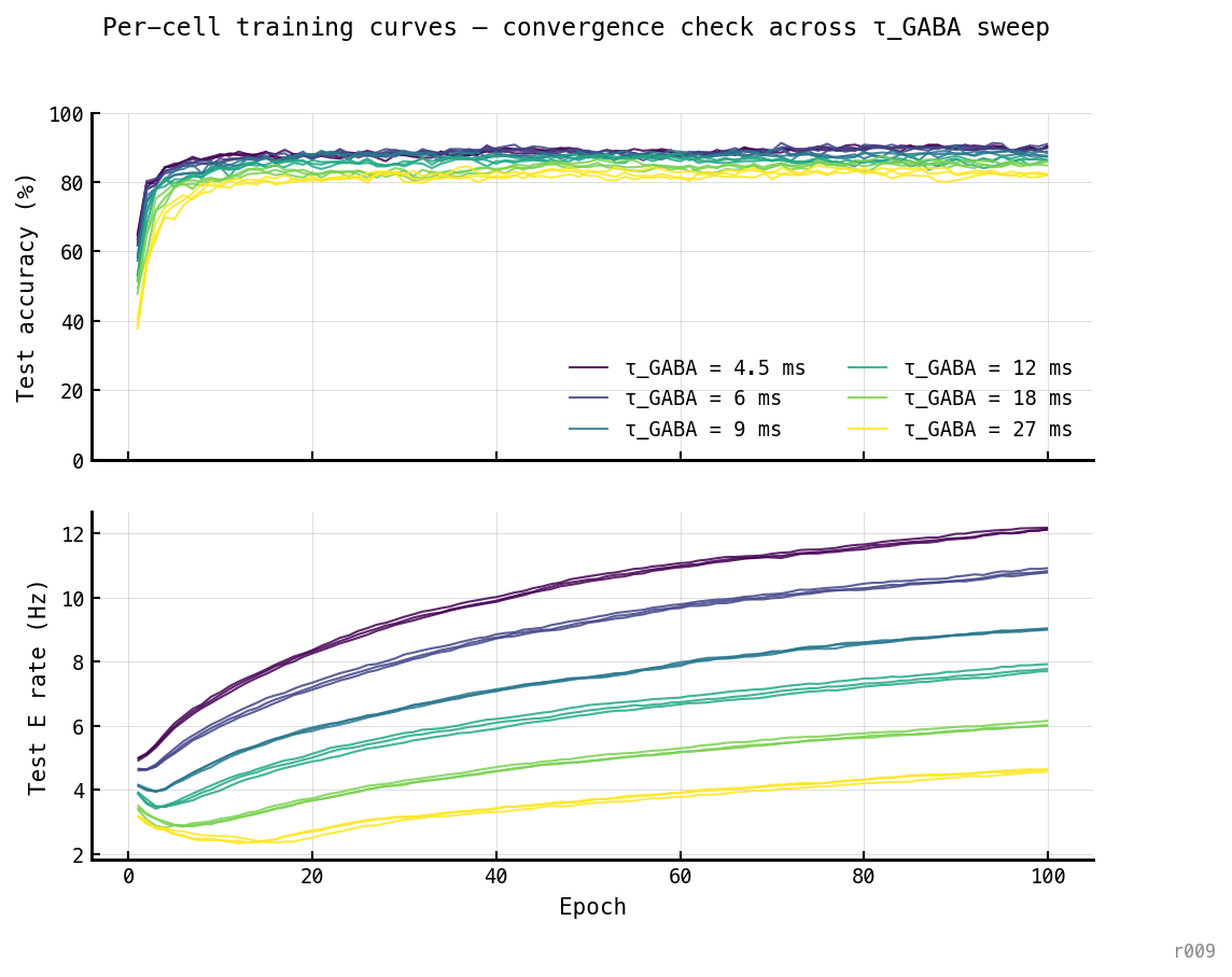
Two stacked panels. Top: test accuracy vs epoch, one line per cell, coloured by τ_GABA. Accuracy plateaus at 80–89% by epoch 15 across all cells. Bottom: test E rate vs epoch — every curve climbs steadily across the first 30 epochs then flattens by epoch 70–100. — Accuracy plateaus by epoch 15; rate keeps climbing until epoch 70–100. The 100-epoch numbers are converged.

training	$a$ (Hz)	$p$ (Hz/Hz)	$R^2$
30 epochs	1.14	0.166	0.990
100 epochs	0.76	0.216	0.997

The shape is robust; $p$ tightens with training. The 100-epoch row is canonical.

Trial-to-trial $f_\gamma$

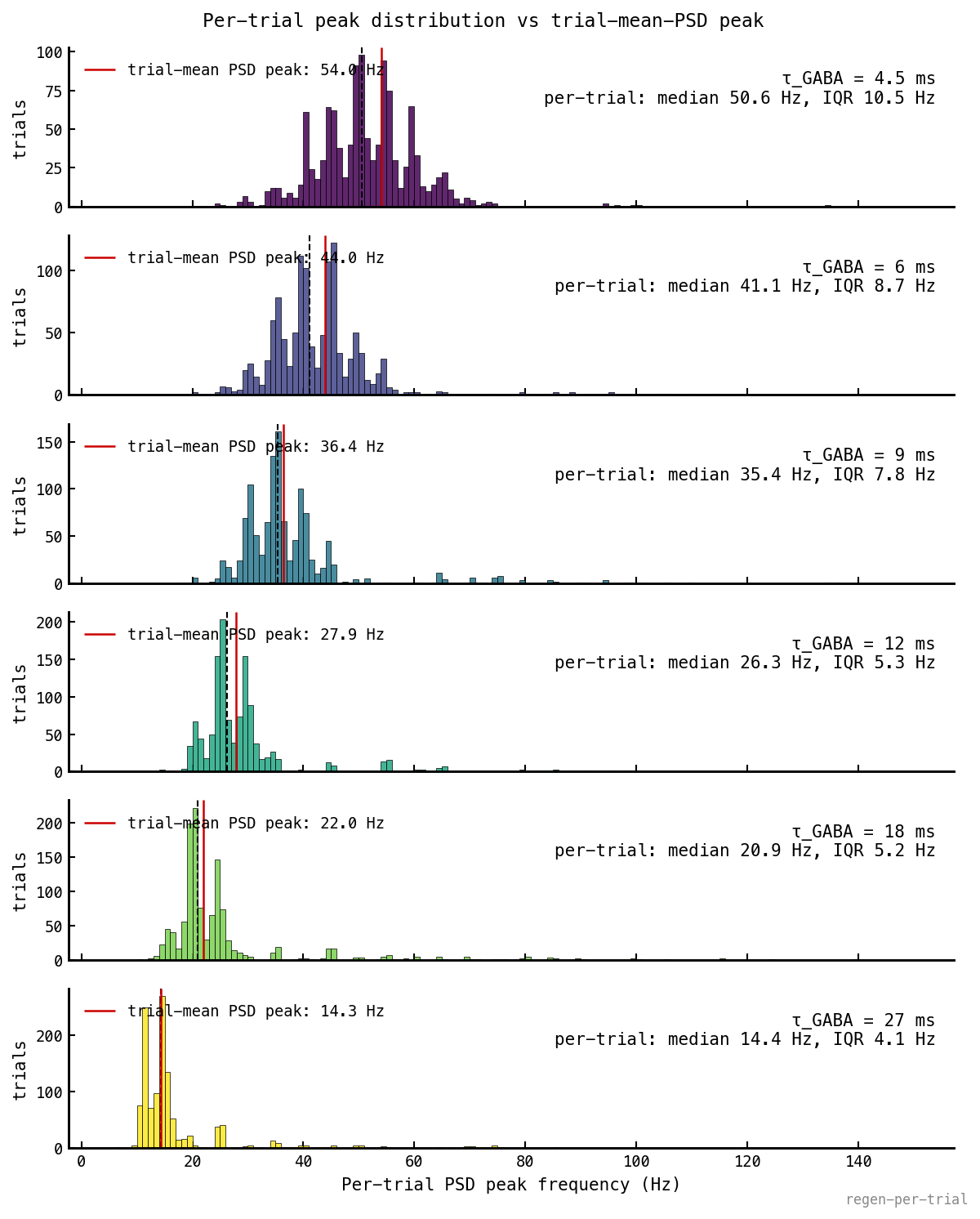
Six stacked histograms, one per τ_GABA value (viridis colormap), of per-trial PSD peak frequencies pooled across the three seeds (1200 trials per panel). Dashed verticals: per-trial medians. Solid red: trial-mean PSD peaks. Distributions have a single-peaked envelope with fine comb-like structure from the 5 Hz Welch bin spacing. — Per-trial peak distribution per $\tau_\text{GABA}$ , pooled across seeds (≈ 1200 trials per panel). Dashed verticals mark per-trial medians; solid red marks the trial-mean PSD peak.

Two read-offs: (a) the trial-mean PSD peak sits 1–3 Hz above the per-trial median (centroid bias of trial-averaging PSDs whose peaks fluctuate), so the per-trial-median refit is the more honest fit; (b) there’s real trial-to-trial spread in $f_\gamma$ that grows with $f_\gamma$ itself.

The comb-like fine structure is a Welch artefact: $\Delta f = 1/T = 5$ Hz quantises each trial’s peak to one of six gamma-band bins, and parabolic interpolation only smears each by $\pm 2.5$ Hz, so per-trial peaks pile up at the bin centres. The comb spacing equals $\Delta f$ exactly — methodological, not physical. The envelope is single-peaked at every $\tau_\text{GABA}$ , ruling out digit-class-specific clusters. A longer $T$ would dissolve the comb.

Population PSDs

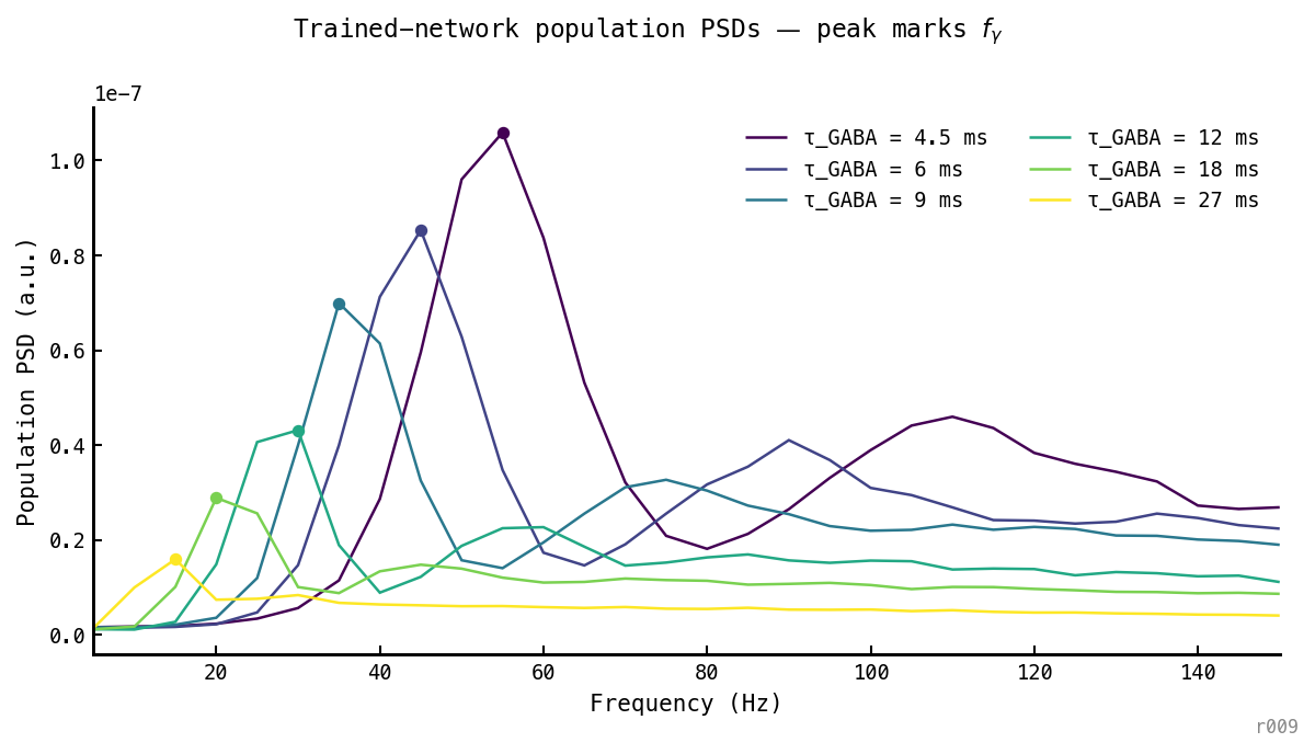
Six PSD curves on a linear y axis, one per τ_GABA value (4.5, 6, 9, 12, 18, 27 ms; viridis colormap), x-axis frequency 5–150 Hz. Each curve has a clear peak in the gamma band, marked with a dot at the parabolic-interpolated peak frequency. — Trial-mean Welch PSDs by $\tau_\text{GABA}$ . Dots mark the parabolic-interpolated peak. Peak shifts cleanly from ≈ 14 Hz at $\tau_\text{GABA} = 27$ ms to ≈ 54 Hz at $\tau_\text{GABA} = 4.5$ ms; no overlap between adjacent conditions.

Parabolic interpolation with peak-bin values $(y_0, y_1, y_2)$ :

f_\gamma = \text{freq}[\text{peak}] + \tfrac{1}{2}\frac{y_0 - y_2}{y_0 - 2y_1 + y_2}\cdot \Delta f, \qquad \Delta f = 5 \text{ Hz}.

Necessary because the bare 5 Hz quantisation would coarsen $f_\gamma$ across the six conditions; on a well-isolated peak the interpolation error is $O((\Delta f)^3)$ .

Single-trial rasters

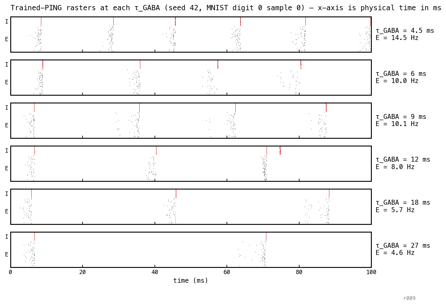
Six stacked raster panels for τ_GABA values 4.5, 6, 9, 12, 18, 27 ms. Each panel shows E spikes (black) and I spikes (red) across the first 100 ms of one MNIST trial. The gamma cycle period grows monotonically with τ_GABA: bursts every ~17 ms at 4.5 ms; every ~63 ms at 27 ms. — One MNIST trial through each network. Cycle period stretches from ≈ 17 ms ( $r_E = 14.5$ Hz) to ≈ 63 ms ( $r_E = 4.6$ Hz). The eye and the spectrum agree.

The affine law

The shape $r_E = a + p \cdot f_\gamma$ is predicted by cycle dynamics, not curve-fitted. Within one cycle of duration $1/f_\gamma$ , a fraction $p$ of E cells emits exactly one spike (those nearest threshold when the I shunt drops); the rest are still recovering. The cyclic per-cell rate is $p \cdot f_\gamma$ . At long $\tau_\text{GABA}$ the I conductance never fully decays and the cycle dissolves into a tonic bath, leaving a feedforward baseline $a$ independent of $f_\gamma$ :

r_E = \underbrace{a}_{\text{feedforward baseline}} + \underbrace{p \cdot f_\gamma}_{\text{cyclic contribution}}.

Top panel: scatter of mean post-training E rate (Hz) vs measured gamma frequency f_γ (Hz). Six clusters, one per τ_GABA value (annotated 4.5–27 ms), three seeds each. Error bars in both dimensions. An affine fit line r_E = 0.76 + 0.216 · f_γ passes through every error bar with R² = 0.997. Bottom panel: test accuracy vs same x-axis — flat at 81–89% across the entire f_γ range. f_γ on the x-axis is the per-trial PSD peak median (see Figure 2). 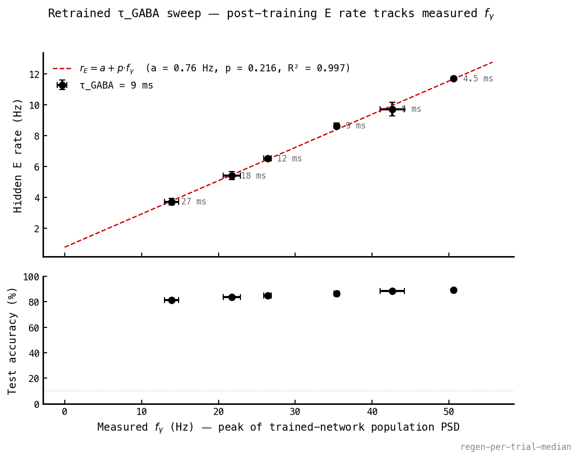— Top: mean post-training E rate vs $f_\gamma$ , six clusters × three seeds, error bars from seed variance. The affine fit passes through every error bar. Bottom: per-cluster accuracy — flat. The rate change is not paid in classification.

Two interpretations come for free:

$p$ is per-cycle participation. At $\tau_\text{GABA} = 9$ ms: $(r_E - a)/f_\gamma = 7.8/35 = 0.22$ , matching the fit. nb024’s per-cell distribution gives 0.21 from a different angle.
$a$ is the non-rhythmic baseline. At $f_\gamma \to 0$ the fit extrapolates to ≈ 0.8 Hz — the no-rhythm regime that nb042 probes directly. The intercept is a prediction, not a nuisance term.

Discussion

nb037 showed rate followed the rhythm under inference-time mutation. nb041 shows the optimiser can’t escape: every retrained network sits on the same affine line.

Cortical prediction

The derivation depends only on the cycle structure produced by the recurrent E↔I loop, not on the task or training substrate. To the extent that cortical pyramidal–interneuron circuits implement the same kind of self-clocking cycle, the law should hold in vivo:

Pyramidal-cell mean firing rate should be linearly predictable from local gamma peak frequency: $r_E \approx a + p \cdot f_\gamma$ , with $p \approx 0.1$ – $0.2$ and a small non-rhythmic baseline $a$ .

Testable in any awake-cortex recording with simultaneous gamma + pyramidal-rate measurement. Falsifiable three ways:

Slope — if $p$ is consistently outside 0.05–0.3, per-cycle participation is the wrong interpretation.
Linearity — if pyramidal rates correlate with gamma power but not gamma frequency affinely, the cycle-counting picture is wrong.
Direction — shortening $\tau_\text{GABA}$ (some benzodiazepine washouts, specific GABA-A manipulations) should raise pyramidal rates, counter-intuitive but a direct consequence.

This assumes adult-cortex-like biophysics ( $\tau_\text{AMPA} = 2$ ms, $\tau_\text{GABA} \in 5$ – $30$ ms, E:I ≈ 4:1). If cortical gamma is generated by a different mechanism (ING, pacemaker-driven), the law need not transfer — so the prediction also tests whether cortical gamma is PING-like.

Next steps

Quantitative-law leg of ar010’s pre-shipping chain. Combined with nb042’s rhythm-locking and dimensional-collapse results, the structural-bound argument is complete.