042 — Perturbations: gamma gates rates not just mean inhibition
Abstract
nb025’s rate gap admits a cheap reading: PING fires less because the I-loop delivers more inhibition. This entry forecloses that reading and identifies what about the I-stream is doing the suppressing — qualitatively (rhythm vs mean), and quantitatively (which temporal precision is required). Scaffolded by ar009 §Leg 1 item 2.
Methods
Pure inference on the trained nb025 PING baseline (seed 42, off). For each batch the I-population spike tensor is recorded from a baseline forward pass, then an override tensor replaces it in a second pass via the nb037 hidden-perturbation hook. The E-population experiences only the override I-stream through ; the readout consumes the perturbed E spikes. Mean per-cell I rate is matched to the baseline to four decimals across every perturbation.
Four perturbation families:
- Baseline — no override; trained PING dynamics.
- Cycle-coherent jitter — partition the trial into blocks of length ( ms at the trained operating point from nb041). For each (trial, block), draw a single Gaussian offset and shift every I-spike in that block by . Within-burst cross-cell synchrony preserved exactly; only the placement of each burst is perturbed. Sweep ms.
- Phase-shuffle — per-trial permutation of the time axis applied to all I-cells together: . Preserves cross-cell co-firing within a timestep; destroys all phase structure.
- Rate-matched Poisson — per-(trial, cell) Bernoulli with . Destroys both temporal and cross-cell structure; tests the variance limit.
Test split from nb025 at medium tier (400 samples, ms, ms, batch 64).
Results
The argument is built in two stages, each identifying a separate architectural variable that holds the rate floor. (1) Cycle-coherent jitter sweeps the burst placement axis and finds the operative timescale is . (2) Per-I-cell jitter sweeps the within-burst synchrony axis and finds destroying synchrony silences E (rather than releasing it), with a much sharper sub-millisecond transition. Each sweep absorbs the corresponding categorical endpoint: full phase-shuffle is the limit of cycle-coherent jitter; rate-matched Poisson is the limit of per-cell jitter.
1. Cycle-coherent jitter — the sweep identifies the operative timescale
Take the trained PING network and apply cycle-coherent jitter to the I-stream at inference: partition the trial into blocks of one gamma cycle, draw a single Gaussian offset per block, and shift every I-spike in that block by . Within-burst synchrony is preserved exactly — bursts move bodily, they do not smear — and the mean I rate is unchanged. At this is the baseline; as grows, bursts are displaced from their phase-locked slots until their placement is decoupled from the gamma cycle. If the operative variable is temporal phase relative to the gamma cycle, the relevant timescale is the cycle period . At the trained operating point ( ms), nb041 gives Hz, predicting the transition at ms.
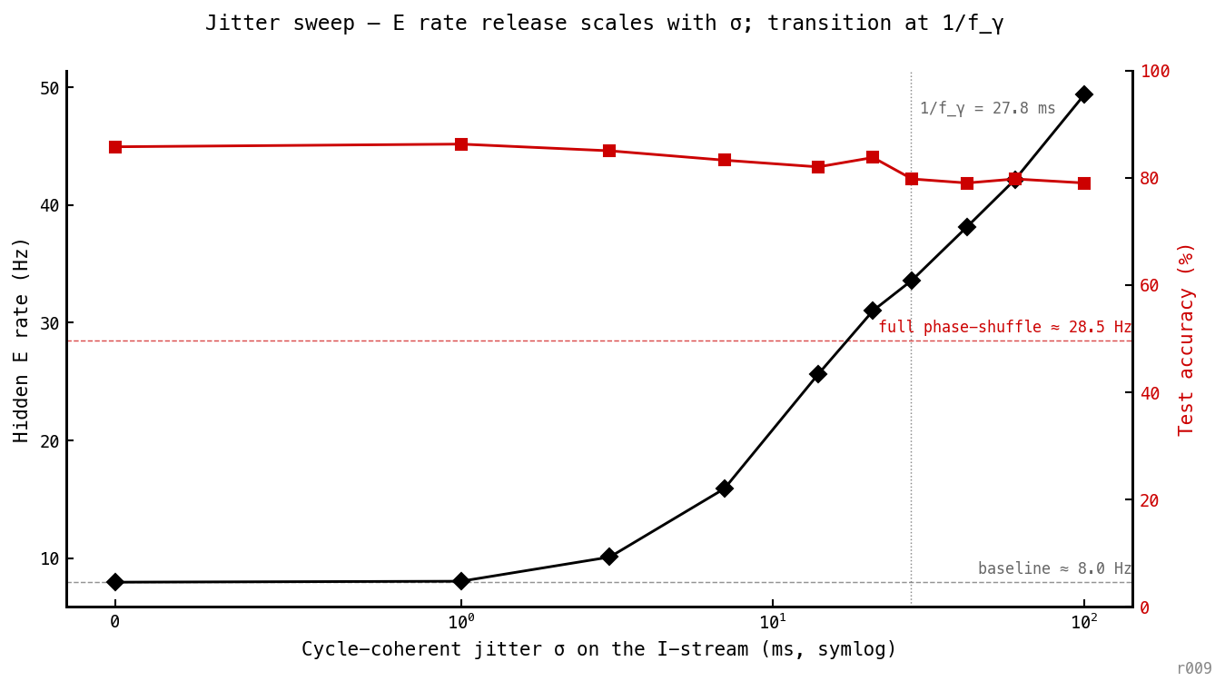
E rate (black) and accuracy (red) vs cycle-coherent jitter , seed 42. Horizontal dashed lines mark the baseline rate ( Hz) and the full phase-shuffle ceiling ( Hz, the asymptote with within-burst structure destroyed). Vertical dotted line at ms — the predicted transition timescale.
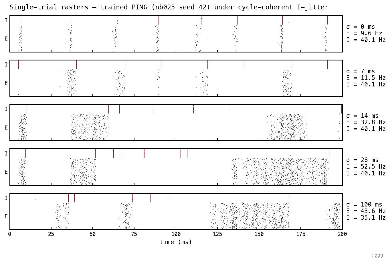
Single trial replayed at five jitter levels (seed 42, MNIST digit 0 sample 0). Per-trial E rate annotated on each panel. The I-bands stay vertical and crisp at every — within-burst synchrony is preserved exactly. What changes is where each burst lands: at larger the bursts get displaced bodily from their phase-locked positions, opening longer gaps in the I-stream that E fires through.
The curve matches the prediction. The rate is flat for ms ( Hz, baseline). The transition is centred between ms and ms, crossing the phase-shuffle ceiling ( Hz) between and ms — just below the predicted inflection. At ms the rate has reached Hz, above the phase-shuffle level because cycle-coherent jitter at very large opens gaps in the I-stream wide enough for E to fire densely with no inhibition at all. Accuracy holds at 79–86% throughout — the rate release is not paid in classification.
What this gets us, beyond the binary “rhythm matters”:
- Identifies the operative timescale. If a different process — refractory dynamics ( ms), membrane time constant ( ms), AMPA decay ( ms) — were the operative clock, the inflection would be elsewhere. It is at .
- The dependence is graded, not knife-edge. The I-loop tolerates sub-cycle jitter and degrades smoothly past it.
- Full phase-shuffle is the asymptote of the jitter sweep, modulo within-burst structure (which is why the ms jitter rate slightly exceeds the phase-shuffle ceiling line — at very large cycle-coherent jitter opens gaps in the I-stream wide enough for E to fire densely with no inhibition at all).
- The transition timescale is a quantitative prediction. is set by nb041’s law. The same architecture trained at a different would give a different , and the jitter inflection should track it accordingly.
2. Per-I-cell jitter — within-burst synchrony is a separate axis
The cycle-coherent sweep moves bursts as whole units, preserving within-burst synchrony exactly. The complementary perturbation is per-spike (per-I-cell) jitter: draw an independent Gaussian offset for every I-spike. Mean per-cell I rate is preserved exactly, burst placement is preserved on average, but the burst itself smears across a window of width ≈ . This tests whether the sharpness of each inhibitory pulse matters, separately from where it lands.
Prediction: if synchrony also matters, the transition should be at ms — the smearing width at which the integrated profile starts looking continuous, the same way a rate-matched Poisson I-stream keeps E silent because never drops low enough for to recover.
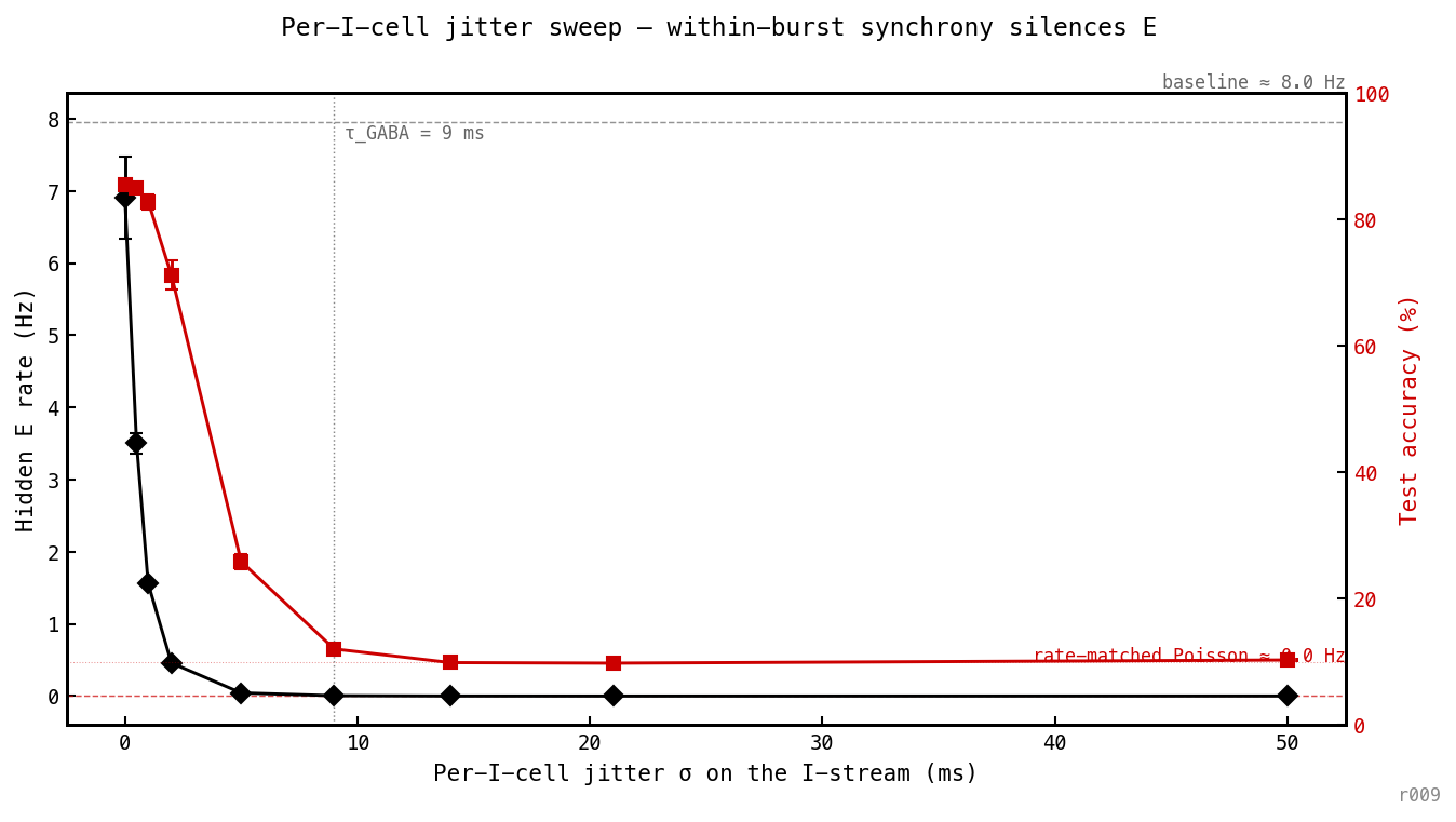
Per-I-cell jitter sweep, three seeds. Each spike receives an independent Gaussian offset; mean per-cell I rate is preserved exactly. E rate (cyan, left axis) falls monotonically from baseline — already halved by ms — and is essentially zero by ms, well below ms. Accuracy (red, right axis) holds at ≈ 85% up to ms, then collapses through 71% (σ = 2) and 26% (σ = 5), bottoming at chance (≈ 10%) by ms. The asymptote is the rate-matched Poisson regime: E silent, accuracy at chance.
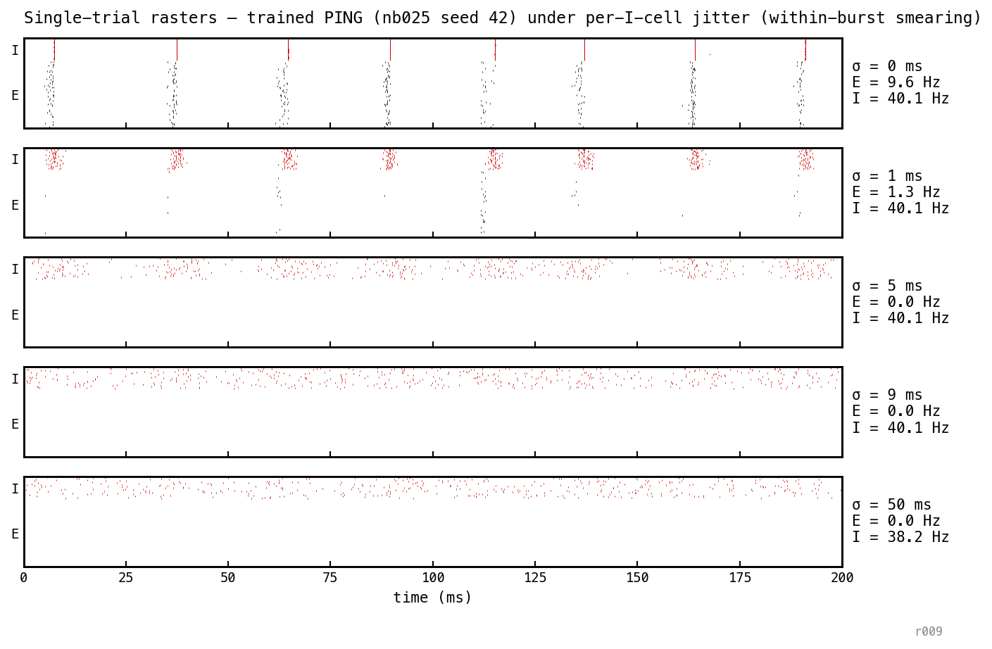
Single trial replayed at five per-cell jitter levels. At the I-bursts are crisp vertical bands. At ms the bursts visibly smear into a few-ms-wide cluster and E firing already collapses to 1.6 Hz. At ms the I-stream looks indistinguishable from a continuous low-variance shunt, and E is silenced. Per-cell jitter doesn’t release E; it destroys the bursty structure that gave E recovery troughs in the first place.
The clean reading: the two jitter regimes test two different things, and the rate floor depends on both.
- Burst placement (cycle-coherent jitter): bursts must land in phase with E activity, with precision ≈ . Destroying placement releases E toward COBA territory.
- Burst sharpness (per-cell jitter): bursts must be sharp enough that has clear troughs between them, with smear width . Destroying sharpness silences E because never drops low enough.
Discussion
The rate floor is held by two independent properties of the I-stream, each tied to a separate transition timescale:
- Burst placement on the gamma cycle, with precision ms. Destroying placement releases E toward COBA territory (cycle-coherent jitter sweep; full phase-shuffle is the asymptote).
- Within-burst synchrony / burst sharpness, with precision ms — in practice the transition is at ms. Destroying sharpness silences E because becomes a continuous shunt with no recovery troughs (per-I-cell jitter sweep; rate-matched Poisson is the asymptote).
Mean inhibition is not the operative variable along either axis. Cycle-coherent jitter at ms releases E to ≈ 49 Hz; per-cell jitter at ms silences E entirely — at identical mean I rates. The “rhythm matters” claim resolves into two more precise claims: bursts must land on phase, and bursts must be sharp.
This integrates with nb041 in a clean way. nb041 retrains PING at different and finds . nb042 (jitter sweep) is the inference-time analogue: keep the trained network, degrade the temporal precision of its I-stream, and watch the rate rise. The transition timescale is set by the same architectural variable that sets the slope of the affine law. Two perturbations through different doors give the same answer: the gamma cycle is the operative clock.
Open question
The jitter sweep’s ms endpoint ( Hz) exceeds the phase-shuffle ceiling ( Hz) and approaches COBA-territory firing. The mechanism (gaps in the I-stream let E fire densely) is mechanistically clear, but the quantitative match between jitter and trained-COBA rates would require comparing matched-rate operating points. Worth probing if the architecture-equivalence claim from nb038 is to be tightened.
Next steps
For ar010: the jitter sweep is now the load-bearing perturbation result. The categorical bar chart becomes a supporting endpoint comparison. A follow-up worth doing — but not on ar010’s critical path — is to retrain PING at a different (say 4.5 ms, giving Hz) and re-run the jitter sweep; the predicted transition should now sit at ms. If the inflection tracks as varies, the quantitative law is independently confirmed by the inference-time experiment.