040 — CUBA-PING

Abstract

nb025–nb038 characterise PING in the conductance-based regime, where every synapse has an exponential filter at $\tau_\text{AMPA}$ or $\tau_\text{GABA}$ . This entry asks whether current-based (CUBA) PING with instant synapses — no synaptic filtering at all — still produces the gamma dynamics and can be trained.

Methods

LIF E and I populations with the same wiring as nb025’s COBA-PING but with no synaptic state: every presynaptic spike at $t-1$ contributes its weight to the postsynaptic current at $t$ and is gone by $t+1$ .

$N_E = 1024$ , $N_I = 256$ , $N_\text{in} = 784$ , $\Delta t = 1$ ms, $T = 200$ ms.
Membrane: $\tau_m = 20$ ms, $V_\text{rest} = 0$ , $V_\text{th} = 1$ , hard reset to $V_\text{rest}$ on spike, $R_m = 1$ . $V$ is floored at $V_\text{rest}$ after each step (membrane can’t fall below the dominant ion’s reversal potential). No refractory period — after reset the cell is free to fire on the next step; the only mechanisms limiting firing rate are membrane decay back to threshold and (in the PING arm) the I-loop suppression.
Weights: $W^{EI} \sim \mathcal{N}(1, 0.1)$ , $W^{IE} \sim \mathcal{N}(1, 0.1)$ , both clamped non-negative; $W_\text{in}$ is 95% sparse with $\mathcal{N}(0, 0.5)$ entries.

V^E_{t+1} = V^E_t + \tfrac{\Delta t}{\tau_m}\!\left(-(V^E_t - V_\text{rest}) + R_m(x_t W_\text{in} - s^I_{t-1} W^{IE})\right), \quad s^E_t = \mathbb{1}[V^E_t \geq V_\text{th}]

V^I_{t+1} = V^I_t + \tfrac{\Delta t}{\tau_m}\!\left(-(V^I_t - V_\text{rest}) + R_m\, s^E_{t-1} W^{EI}\right), \quad s^I_t = \mathbb{1}[V^I_t \geq V_\text{th}]

Both arms — full PING and the E-only ablation — go through oscilloscope train --model cuba-ping ... and --model cuba-noping ... respectively; recipe, optimiser, surrogate gradient, TBPTT window, batching, and seed all match. The output layer is a non-spiking LIF integrator ( $\tau_\text{out} = 20$ ms) whose time-averaged membrane is the logits — so silent hidden activity gives a flat output and no class signal. The hidden layer is forced to spike for the readout to carry any information.

Results

Untrained dynamics

Fixed weights, no training. Spatially uniform Poisson input at 80 Hz per channel for the full 200 ms window.

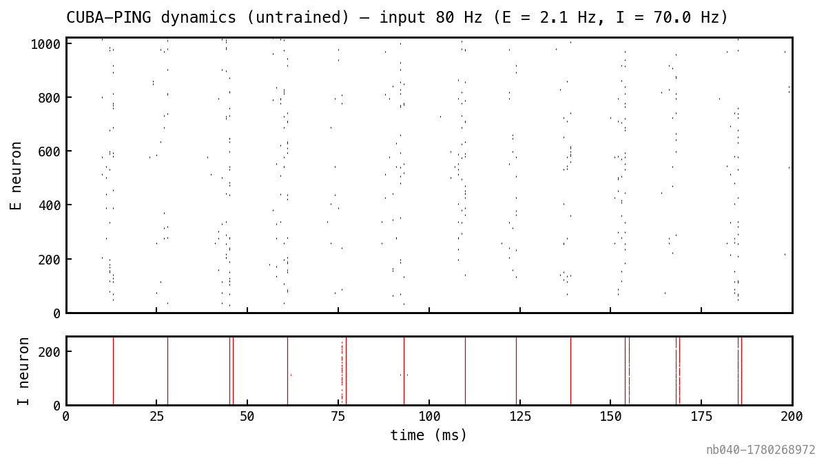
Two-panel raster of CUBA-PING at uniform 80 Hz Poisson input. E neurons fire in sparse, time-locked bursts; I neurons fire in narrow synchronous bursts immediately following each E burst. — Spike raster from one trial with fixed random weights and uniform 80 Hz Poisson input on every channel. E above (black), I below (red). I shows narrow synchronous bursts at gamma cadence; E bursts immediately precede each I burst.

Recruitment threshold, inhibitory clamp on the E rate, periodic E→I bursts — the architectural signatures of PING survive without any synaptic filter. The cycle period is set jointly by $\tau_m$ and the time it takes the input drive to push enough E cells back above threshold for the next round.

Training CUBA-PING

$W_\text{in}$ and $W_\text{out}$ trainable, frozen $W^{EI}$ and $W^{IE}$ . Surrogate-gradient BPTT on Poisson-encoded MNIST. Adam at lr $2 \times 10^{-3}$ , batch 64, mem-mean output readout, TBPTT window $K = 10$ . The $K = 10$ window is load-bearing — full BPTT diverges (Section BPTT stability below).

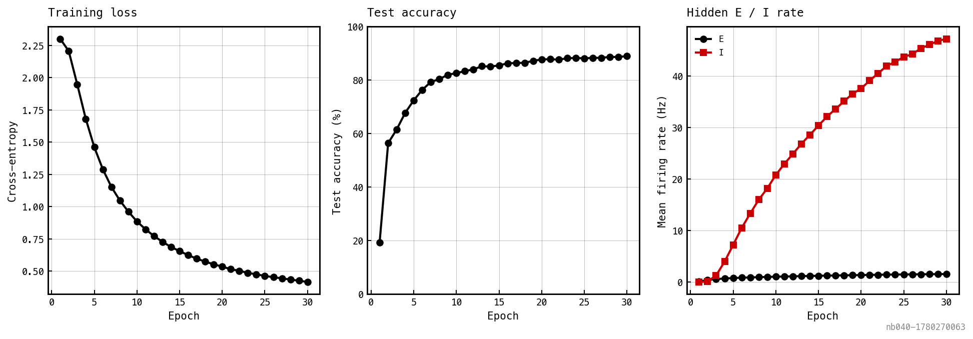
Three panels: training cross-entropy loss decreasing, test accuracy climbing past chance, and hidden E (black) / I (red) firing rates climbing slowly. — Cross-entropy loss (left), test accuracy (middle), and mean hidden E (black) / I (red) rates (right). The I-loop suppresses E to ≈1 Hz while the readout drives accuracy upward. Headline numbers above reflect the run that produced these figures.

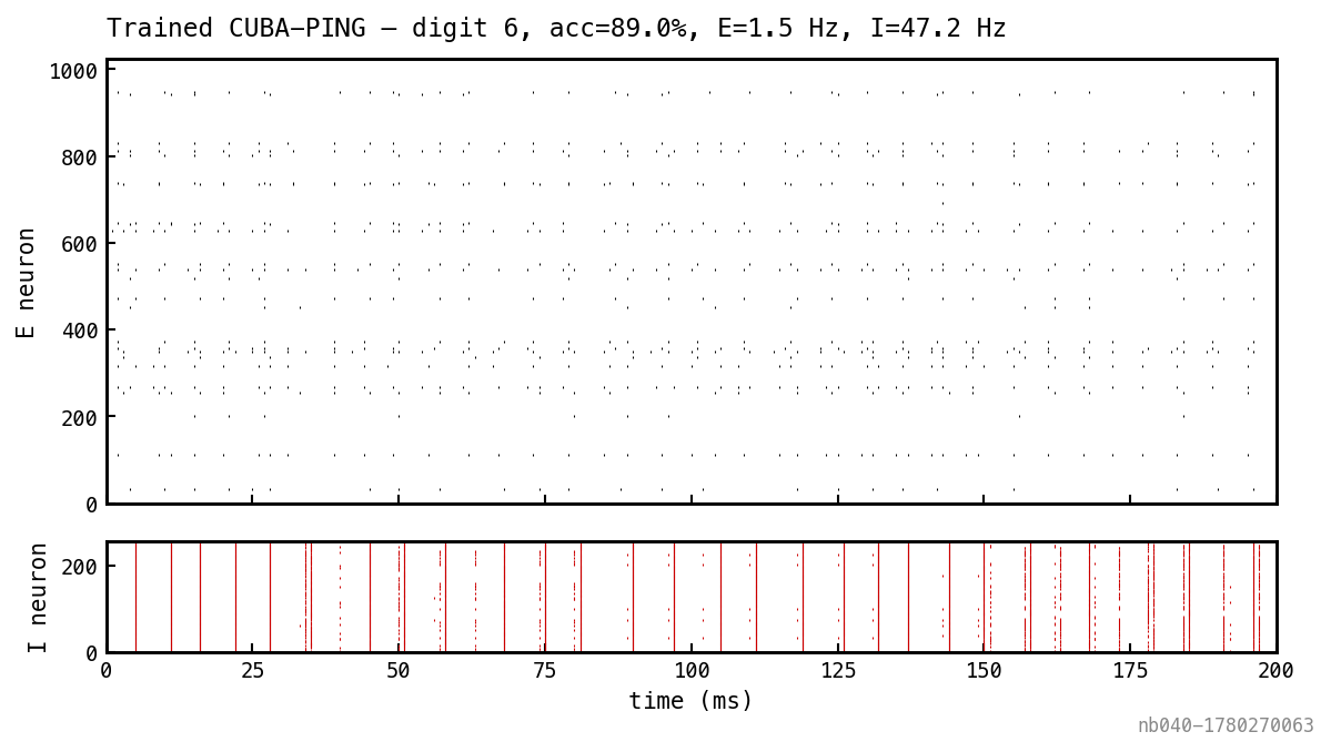
Two-panel raster of the trained network replayed on a single test trial. E neurons fire sparsely; I neurons fire in periodic bursts. — One MNIST test sample replayed on the trained network. Untrained PING dynamics (Figure 1) survive — E spikes are sparse and digit-selective; I bursts at gamma cadence.

CUBA-no-PING ablation

The interesting question is why CUBA-PING ends up at sub-Hz E rates. Two candidates:

The I-loop clamps the rate. Inhibitory feedback suppresses E whenever it gets recruited; the optimiser finds a sparse-spike solution. PING is necessary.
The mem-mean readout doesn’t need spikes. A continuous membrane readout can classify from $V^E$ patterns directly. PING is incidental — any CUBA LIF stack would do.

The control: a CUBA no-PING network (E-only, no $W^{EI}$ , no $W^{IE}$ , no I population), same recipe as above.

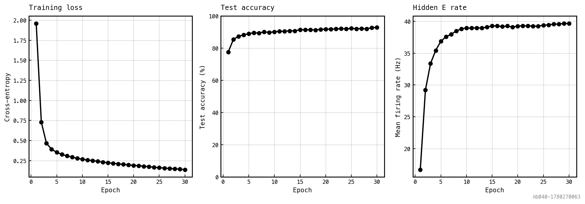
V^E_{t+1} = V^E_t + \tfrac{\Delta t}{\tau_m}\!\left(-(V^E_t - V_\text{rest}) + R_m\, x_t W_\text{in}\right), \quad s^E_t = \mathbb{1}[V^E_t \geq V_\text{th}]

Three panels: training cross-entropy loss decreasing fast, test accuracy climbing past 80%, and hidden E rate climbing to tens of Hz. — Same axes as Figure 2 minus the I-loop. The E rate climbs immediately into the tens of Hz; accuracy converges within a handful of epochs.

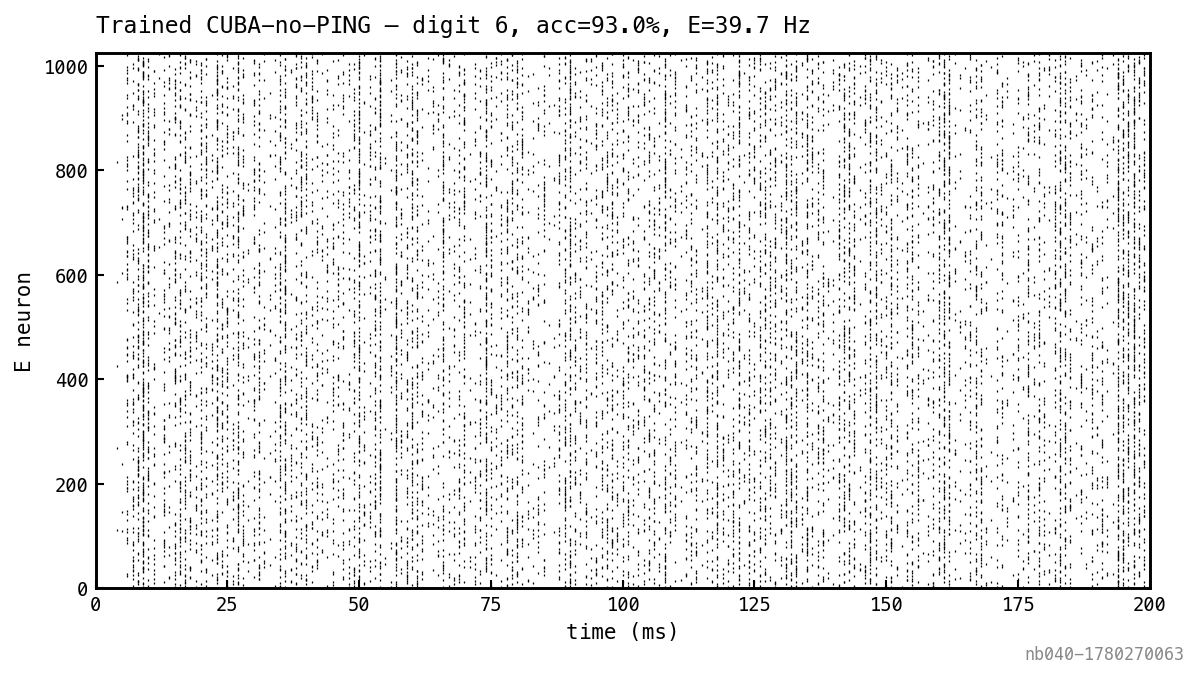
Single-panel raster of the trained CUBA-no-PING network on one MNIST test trial. — E spike raster for one MNIST test trial after training. No I population to render. Compare to Figure 3 — the trained network is dense-spiking across the trial rather than sparsely bursting.

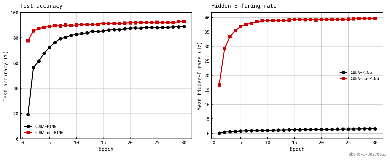
Two panels: test accuracy and hidden E firing rate for both arms over training. — Black: CUBA-PING. Red: CUBA-no-PING. The rate curves diverge by an order of magnitude; the accuracy gap is bounded.

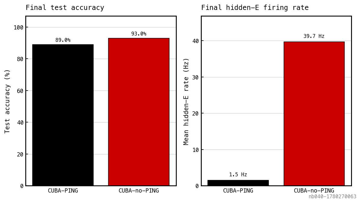
Two bar-chart panels comparing final test accuracy and final hidden-E firing rate for CUBA-PING (black) and CUBA-no-PING (red). — Final test accuracy (left) and mean hidden-E firing rate (right) at the end of training. The same axes as Figure 6 collapsed to single numbers — the rate-accuracy trade in headline form.

Both effects of the I-loop show up cleanly:

The rate clamp is real and strong. Removing the I-loop lets the E rate climb into the tens of Hz — biologically high but within the snnTorch / rate-coded SNN regime. The I-loop in place holds the rate near 1 Hz: an order-of-magnitude sparsification with no $L_\text{rate}$ regulariser.
The sparsification has a real but bounded accuracy cost. Roughly 4 pp at large tier. The output-LIF readout integrates spike events, so suppressing E spikes throttles the output membrane response; the network still has enough integrated signal to classify, just less than the dense-spike control.

This is the same tradeoff the COBA-PING baselines in nb025 Figure 5 walk via the $\theta_u$ spike-budget term — except CUBA-PING walks it by the architectural inhibitory clamp rather than by an explicit penalty.

BPTT stability

The single design choice in the training section that takes some justification is the TBPTT window. With $K = 10$ the network trains; with $K = T = 200$ (full BPTT) gradients overflow to NaN within the first batch.

The recurrent Jacobian

The loss depends on $\{s^E_t\}$ via the output-LIF integrator. By the chain rule the gradient on $W_\text{in}$ accumulates $\partial L / \partial V^E_t$ at every step, and that backward signal routes through s_E and s_I via the I-loop even though the forward readout doesn’t.

One E→I→E round trip:

V^E_t \xrightarrow{\text{spike}} s^E_t \xrightarrow{V^I \text{ update}} V^I_{t+1} \xrightarrow{\text{spike}} s^I_{t+1} \xrightarrow{V^E \text{ update}} V^E_{t+2}

Four Jacobian links: surrogate at E (bounded by $\sigma$ , the surrogate slope), E→I drive ( $\alpha R_m\, W^{EI}$ with operator norm $\alpha R_m \|W^{EI}\|$ ), surrogate at I (bounded by $\sigma$ ), I→E suppression ( $\alpha R_m\, W^{IE}$ with operator norm $\alpha R_m \|W^{IE}\|$ ). Multiplying:

\left\|\frac{\partial V^E_{t+2}}{\partial V^E_t}\right\|_{\text{loop}} \leq (\alpha R_m)^2\, \sigma^2\, \|W^{EI}\|\, \|W^{IE}\|

For random matrices with entries $\mathcal{N}(\mu, \sigma_w)$ the spectral norm is well-approximated by $\mu \sqrt{\min(N_\text{pre}, N_\text{post})} + O(\sigma_w \sqrt{\max(N_\text{pre}, N_\text{post})})$ :

$W^{EI}$ , $W^{IE}$ at $\mathcal{N}(1, 0.1)$ , shape $1024 \times 256$ or transpose: $\|W\| \approx \sqrt{256} \cdot 1 + 0.1 \sqrt{1024} \approx 19$ .
$(\alpha R_m)^2 \sigma^2 \|W^{EI}\| \|W^{IE}\| \approx (0.05)^2 \cdot 19 \cdot 19 \approx 0.9$ .

Just under unity at this recipe — but with moderate spectral slack the per-cycle factor exceeds 1 and growth begins. Over $T = 200$ steps the compound overflows float32 well before the trial ends, so full-horizon BPTT is unreliable in practice.

Why truncated BPTT works

TBPTT with window $K$ caps the per-cycle compound to $K/2$ round trips instead of $T/2$ . The per-step factor raised to $K/2 = 5$ is finite and well within float32. More importantly, the consistently-signed suppression signal is now summed over $K = 10$ steps instead of $T = 200$ , so its magnitude is comparable to the readout signal and the optimiser sees a balanced gradient.

The cost is bias. TBPTT computes the gradient as if each window were independent. This is wrong — $V^E$ at step 10 really does depend on $V^E$ at step 1 via membrane decay. For 200 ms MNIST trials this bias is negligible; for sequence tasks with genuine long-range structure (language modelling, sequence MNIST), TBPTT would underestimate long-range gradients and systematically miss those features. Calling it “truncated” is a bit unfair — the truncation isn’t a bug, it’s the regulariser that lets you train at all. Local-BPTT or gradient horizon limit would be a more honest name.

Discussion

The instant-synapse CUBA-PING has the right dynamics without any synaptic filtering (Figure 1), is trainable when (a) the readout is an output-LIF mem-mean that requires hidden spikes to flow and (b) the BPTT horizon is limited to a few times $\tau_m$ , and is ablation-checked: removing the I-loop raises the E rate by an order of magnitude at a bounded ≈4 pp accuracy cost. Both arms go through the same oscilloscope code path, so the only difference between Figures 2/3 and Figures 4/5 is the I population’s presence.

Next steps

Scale to full MNIST. Training loss is still decreasing at the end of the medium-tier run, so the operating point is not yet converged. Full MNIST + more epochs should close the gap to the COBA-PING baselines.
Add an explicit $L_\text{rate}$ like nb025’s, exposing a $\theta_u$ knob that lets you slide along the rate–accuracy frontier on top of what the architecture already gives.
Replace TBPTT with a principled stabiliser — spectral normalisation of $W^{EI}$ / $W^{IE}$ , or a Jacobian-norm regulariser — that lets full-horizon BPTT through and closes the COBA-PING gap from below.
Add a refractory window ( $\approx 1.5$ ms for E, $\approx 0.5$ ms for I, matching the COBANet baselines). The current model has none, which gives every cell an unbounded firing-rate ceiling and likely contributes to the no-PING control’s ≈70 Hz E rate. With refractory in place that ceiling drops to $1/(\tau_\text{ref}) \approx 667$ Hz for E cells; the no-PING upper rate would compress, narrowing the rate gap to the PING arm without changing the qualitative comparison.