048 — Trained PING streams sequential digits without retraining
Abstract
Can a network trained one-digit-at-a-time on 200 ms trials classify a stream of digits at ms each, without retraining? At ms (≈ 2 gamma cycles) all five sequential MNIST digits classify correctly, with cycle-locked sparse spiking and a readout that flips within one cycle of each transition. A 2D sweep over shows a sub-cycle failure floor at ms and a broad high-accuracy plateau above it where short presentation time and weak drive trade off cleanly along iso-accuracy diagonals.
Methods
Networks. Canonical nb025 PING baselines at off, three seeds (42, 43, 44), medium tier (1600 train / 400 test, 100 epochs). Inference-only at the trained ms; the 2D sweep averages over the three seeds, single-trial demos use seed 42.
Stream construction. Sample MNIST test digits, encode each as a Poisson spike train for ms at the given input rate, concatenate along time. Digit transitions are hard switches — the Poisson rate flips instantaneously at . The network processes the full stream in one forward pass. The 2D sweep covers ms × input rate Hz per channel, with 40 streams × 10 digits per cell (1200 segments per cell, 3 seeds).
Readout. Same output LIF, same , same with ms. The only difference from training: a sliding-window mean of width ms replaces the full-trial integration.
Per-segment prediction is read at the end of each -window.
Results
Headline: 5 digits at ms
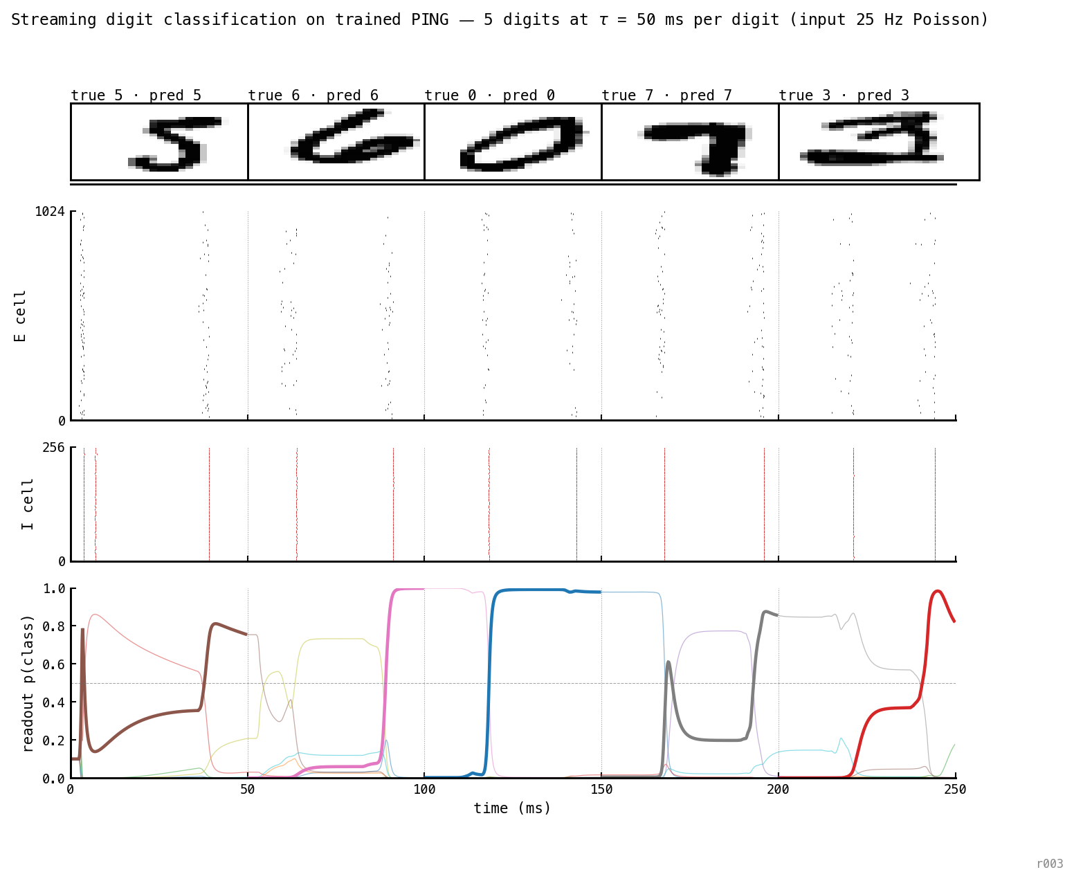
Five sequential digits (5, 6, 0, 7, 3) at ms each — ≈ 2 gamma cycles per digit, 250 ms total. Gamma cadence (≈ 28 ms) is preserved across the stream. The readout flips to the new digit within one cycle of each transition and reaches near 1.0 by the segment’s end. 5/5 correct.
Varying stream
A stronger test: vary both knobs within a single stream so each digit gets its own duration and input rate.
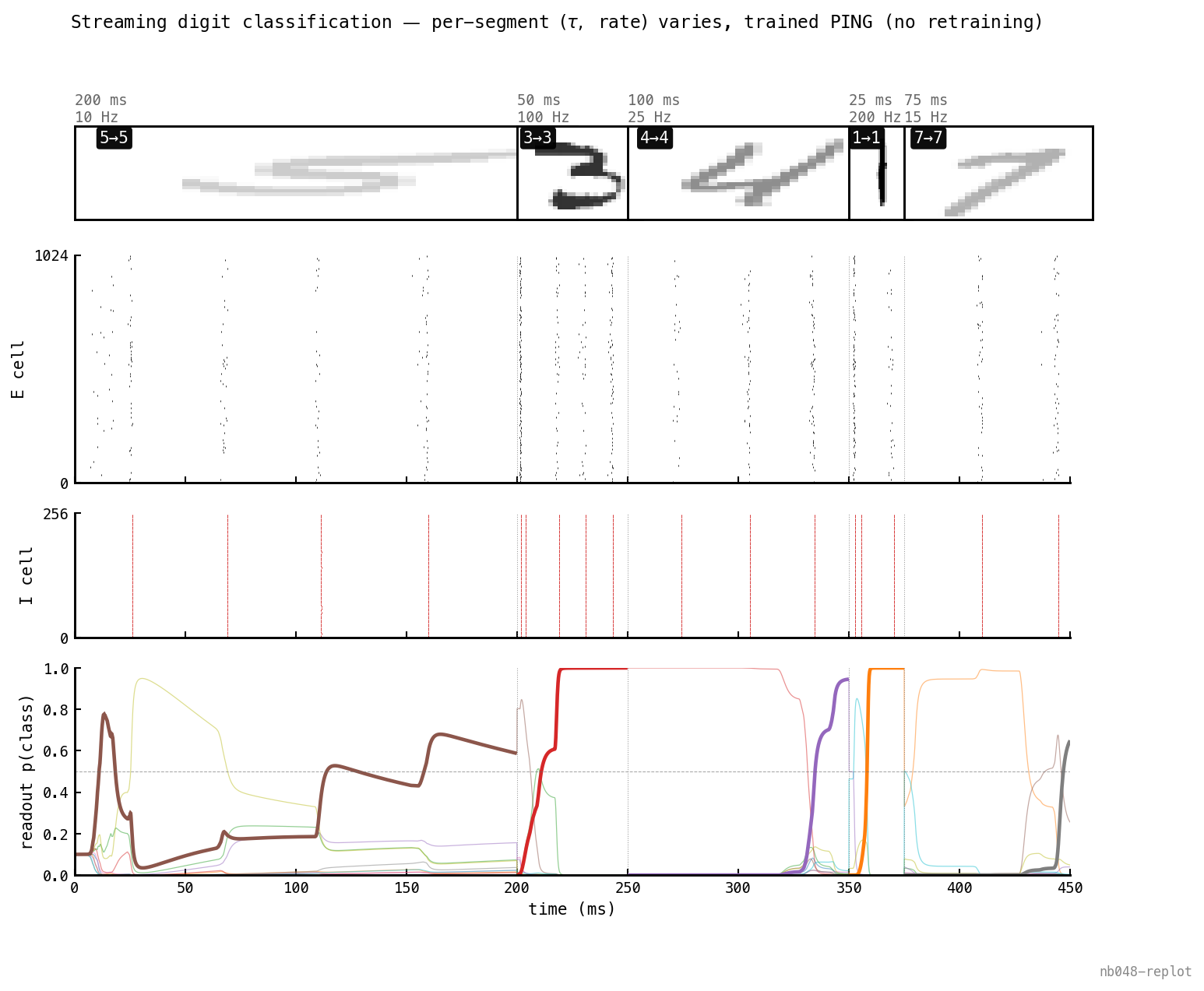
5/5 with varying within a single stream — durations 25–200 ms, rates 10–200 Hz. Thumbnail opacity ∝ input rate (faint = weak drive, bold = strong). The sliding window uses each segment’s own , so each digit’s prediction respects its presentation window.
Accuracy across the grid
To map the operating regime quantitatively, sweep and input rate independently and report per-segment accuracy.
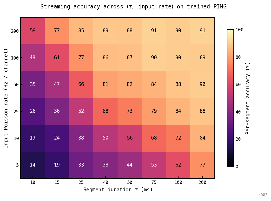
8 × 6 = 48 cells, 3 seeds × 1200 segments per cell. Extended down to ms (≈ 0.36 of a gamma cycle) to resolve the sub-cycle failure regime.
Three observations:
- Sub-cycle failure below ms. At ms even 200 Hz input only reaches 59% — the architecture cannot classify within less than one cycle regardless of drive. This is the cleanest evidence that the gamma cycle is the temporal quantum of the trained network’s classification ability.
- Above one cycle, accuracy ≈ . Iso-accuracy contours run diagonal in log-log space; and input rate substitute for each other once the cycle quantum is cleared. Boosting input rate compensates for short presentation time and vice versa.
- The trained cell at 88% is interior to the plateau — corner cells gain only 3 pp. Substantial headroom in both directions at the trained operating point.
Discussion
The headline figure makes four claims simultaneously visible: sparseness in the E raster, cycle locking in the I-burst clock, class-tracking readout probabilities, and re-identification within ≈ 1 cycle of each digit switch. The trained PING dynamics carry per-cycle class information, and the sliding-window readout — the only change from the training-time readout — surfaces that information at the per-segment timescale.
For the rate-floor story in ar009 / ar010: the architecture’s per-cell rate is bounded by (nb041, nb046). The grid says that with enough drive the network can classify within roughly one cycle — per-cycle information density is sufficient for the task. The bound is tight but not crippling.
Two caveats:
- Sliding-window ≠ trained readout. Same output LIF and , only the integration window changes. A streaming-specific retrain could do better; the point here is that the already-trained network is functional in this regime without any new gradient.
- Hard switches, not cross-fades. Real continuous-input regimes (speech, video) blend transitions; we don’t test that.
Next steps
- Train on streaming data. Does a network trained with ms segments and a sliding readout outperform post-hoc streaming on the medium-tier baseline?
- Cross-fade transitions. Replace hard switches with 10-ms blends; quantify the network’s transient-response time directly.
- interaction. If changes the cycle period (per nb041), does the streaming sweet-spot scale linearly with it?
- COBA control. Run the same protocol on a trained COBA baseline (no gamma cycle) to ask whether anything here is PING-specific, or just a property of any trained mem-mean readout.