049 — Gradient descent prunes PING via Dale's-law clamping (trains)

Abstract

In nb025 the recurrent inhibitory weights $W^{EI}, W^{IE}$ are frozen at biophysical values — the gamma loop is treated as anatomy, not as something training can touch. If we unfreeze them, does Adam rediscover the same loop? No. The frozen control trains to canonical PING ( $E \approx 8$ Hz, $I \approx 38$ Hz, $f_\gamma \approx 38$ Hz, 86% test accuracy). Every trainable condition — whether started at canonical PING values, at zero, or at 10% of canonical — collapses to dense E firing with the I population silent, at 88% accuracy. The mechanism is Dale’s-law-mediated pruning: Adam drives most $W^{EI}$ entries below zero, the forward-pass clamp turns them into structural zeros, and the loop is gone. PING is a structural prior the architecture imposes through the freeze, not one gradient descent recovers on its own.

Methods

Architecture. $N_E = 1024$ excitatory, $N_I = 256$ inhibitory, mem-mean readout, Dale’s law enforced. Hyperparameters match the nb025 PING baseline: Adam at lr $4 \times 10^{-4}$ , batch 256, surrogate slope 1, $W_\text{in} \sim \mathcal{N}(1.2, 0.12)$ at 95% sparsity, gradient norm clipped to 1.0, $\Delta t = 0.1$ ms, $T = 200$ ms, no firing-rate regulariser.

Sweep. Four conditions × three seeds (42, 43, 44) on the medium tier (1600 train / 400 test MNIST, 100 epochs). Only the initial $(W^{EI}, W^{IE})$ and the trainable-or-not flags vary across conditions.

Condition	$W^{EI}, W^{IE}$ init	Trainable?
frozen_ping (control)	canonical biophysical	no
trainable_ping_init	canonical biophysical	yes
trainable_zero_init	$0$ (COBA-equivalent start)	yes
trainable_small_init	$0.1 \times$ canonical	yes

Canonical biophysical means $W^{EI} \sim \mathcal{N}(1.0, 0.1)$ μS, $W^{IE} \sim \mathcal{N}(2.0, 0.2)$ μS at $N_I = 256$ , fan-in-normalised — so the trainer reports per-edge means of ≈ 0.0010 and ≈ 0.0078.

Results

Each condition gets two paired figures: a diagnostic card (training trajectories on top, final E PSD bottom-left, single-trial raster bottom-right) and a weight-distribution card (histograms of $W^{EI}$ and $W^{IE}$ entries, init outline vs trained fill). The histograms show effective values — stored entries with $w < 0$ are clamped to zero before histogramming, so the Dale’s-law-pruned majority piles up in the first bin and surviving entries form the right-hand tail. Legends report the post-clamp mean and the pruned fraction.

Frozen PING (control)

Diagnostic card for the frozen control. Top strip: |W_ei|_F and |W_ie|_F are flat across all 100 epochs (frozen by construction). E rate climbs from ≈ 7 Hz at epoch 1 to ≈ 9 Hz; I rate climbs from ≈ 11 Hz to ≈ 38 Hz. Accuracy reaches 86% by epoch 20 and plateaus. Bottom-left: PSD with a clean gamma peak at ≈ 38 Hz. Bottom-right: single-trial raster shows visible gamma bursts at ≈ 28 ms cadence in both E and I populations. 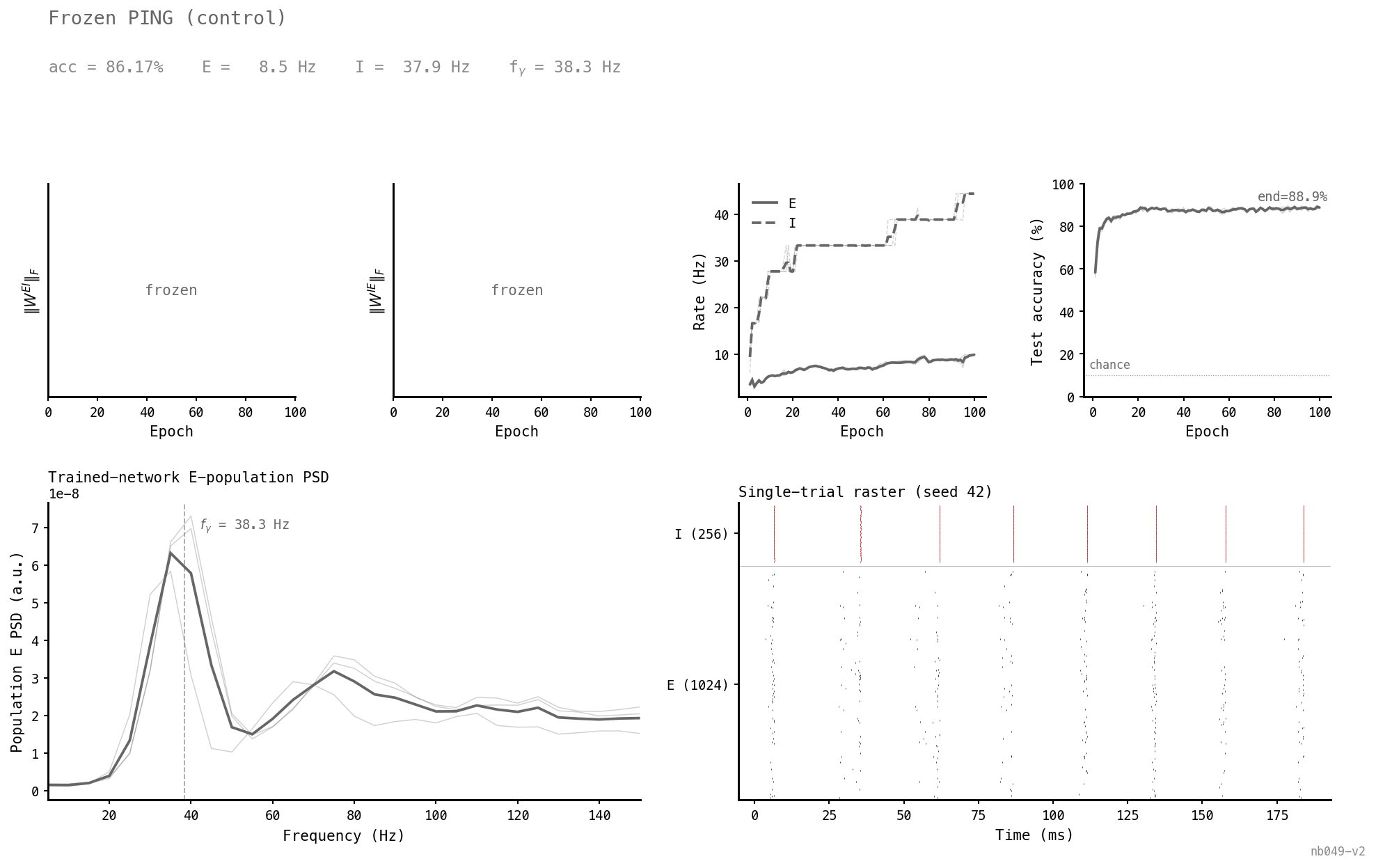— Recurrent weights stay at canonical. E and I rates settle at ≈ 8.5 / 38 Hz, the PSD has a clean gamma peak at 38 Hz, the raster shows cycle-locked bursts. 86.2% test accuracy. This is the reference for what “PING is on” looks like.

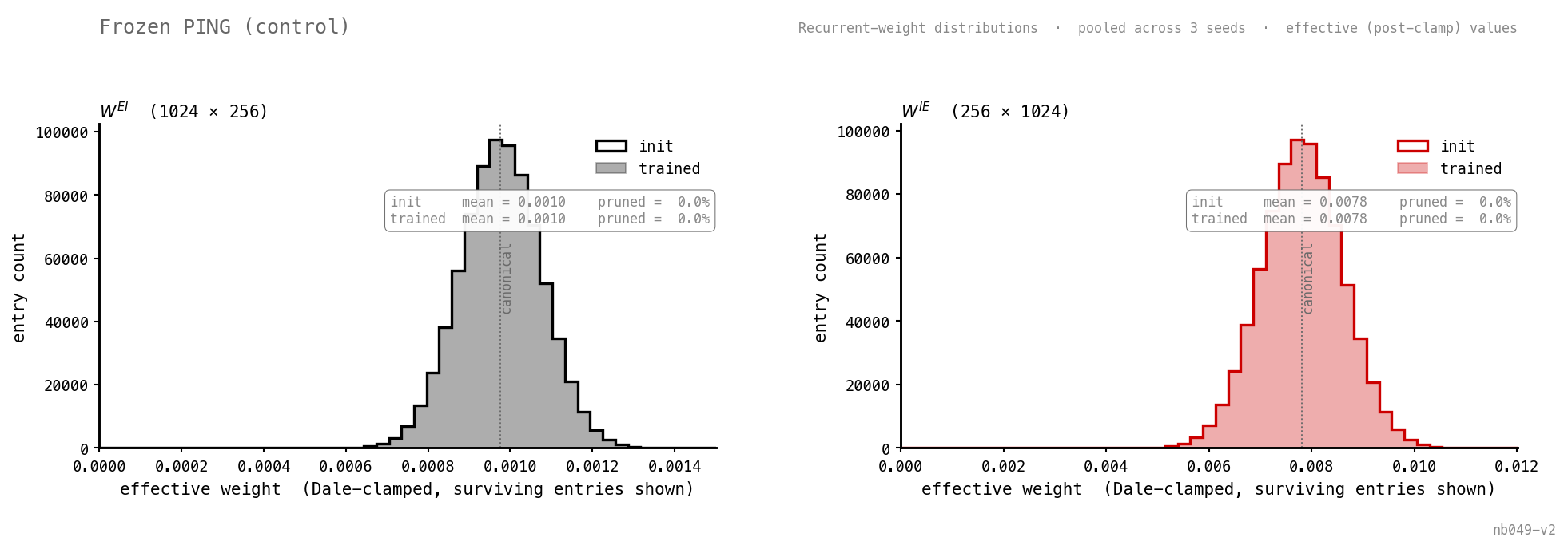
Two-panel histogram. Left: W^EI ≈ 260,000 entries, init outline and trained fill overlap exactly, distribution centred at ≈ 0.0010, 0% pruned. Right: same for W^IE, centred at ≈ 0.0078, 0% pruned. — Init and trained distributions overlap exactly. The sanity check: nothing about the recurrent loop moves.

Trainable, PING initialisation

Diagnostic card. Top strip: |W_ei|_F drifts from canonical 0.0010 toward higher absolute-value Frobenius means; |W_ie|_F barely moves. E rate climbs from ≈ 8 Hz to ≈ 42 Hz over the first 20 epochs; I rate collapses from ≈ 11 Hz to ≈ 0 within ≈ 15 epochs. Accuracy reaches 88% by epoch 25 and plateaus. Bottom-left: PSD peak shifted to ≈ 55 Hz with reduced low-frequency mass. Bottom-right: single-trial raster shows dense asynchronous E firing across the entire trial; the I row is essentially empty. 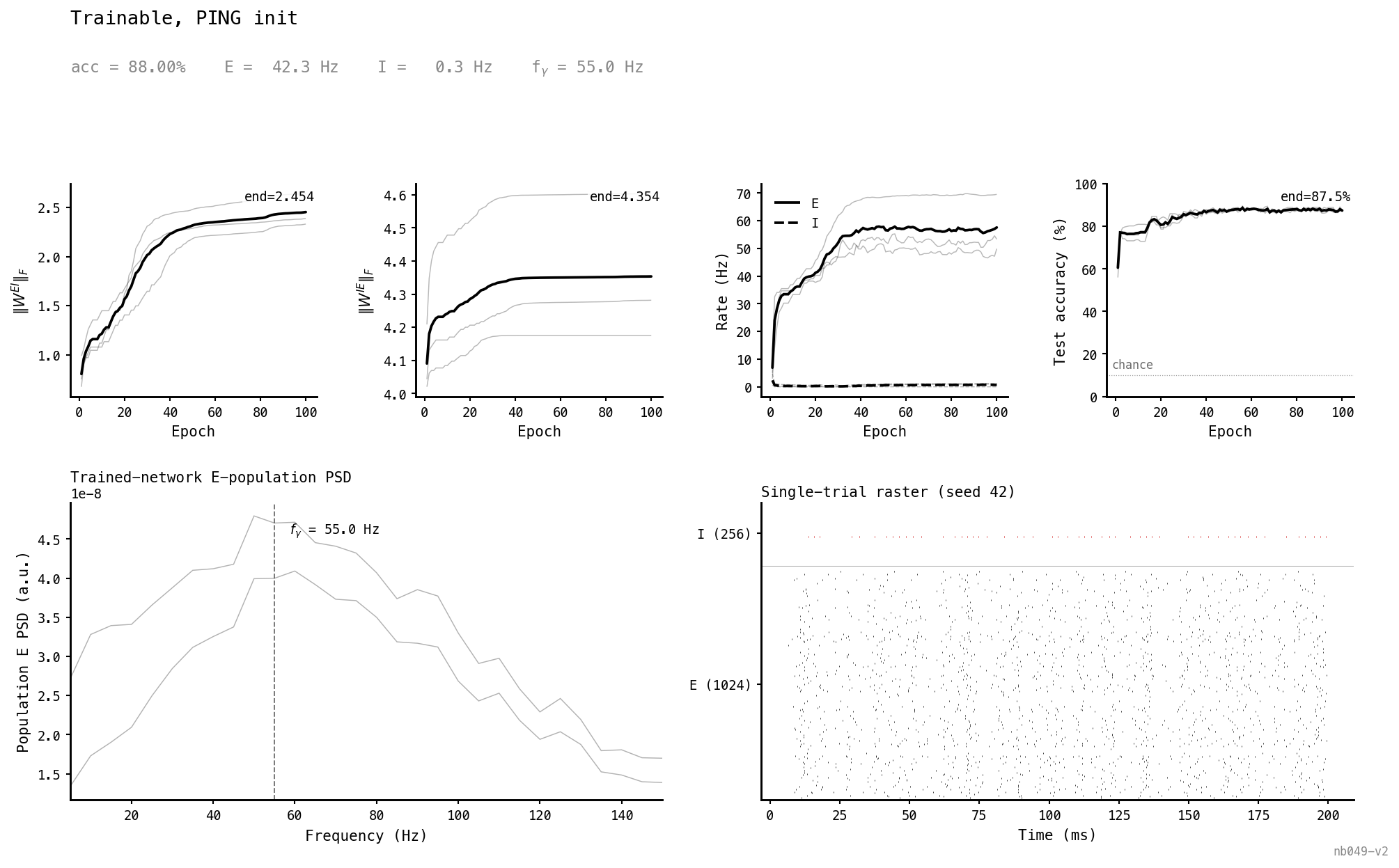— Start the trainable recurrent matrices at the canonical PING values and let them go. Within 15 epochs the I population is silent, E saturates near 42 Hz, the gamma peak drifts up to ≈ 55 Hz, and the raster shows dense asynchronous E firing. 88.0% accuracy — about 2 pp above the frozen control.

Two-panel histogram (effective weight, w<0 clamped to 0, pooled across 3 seeds). Left: W^EI init outline is the canonical half-normal centred near 0.0010, 0% pruned. Trained fill is broader, shifted into a sparse positive tail reaching ≈ 0.016. 73% of entries are pruned to zero; the effective post-clamp mean drops to ≈ 0.0005, lower than the init's 0.0010. Right: W^IE init and trained distributions overlap closely at ≈ 0.0078, 0% pruned. 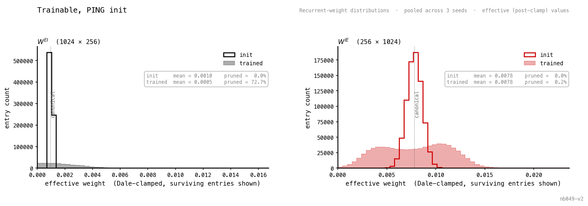— Why the loop dies: **73% of $W^{EI}$ entries are pruned** (Adam pushed them below zero, the forward-pass clamp made them structural zeros). The surviving 27% grew, but the post-clamp mean dropped to 0.0005, *below* the init’s 0.0010. $W^{IE}$ barely moves. Most I cells lose their drive, the gamma shunt that paces E firing vanishes.

Trainable, zero initialisation

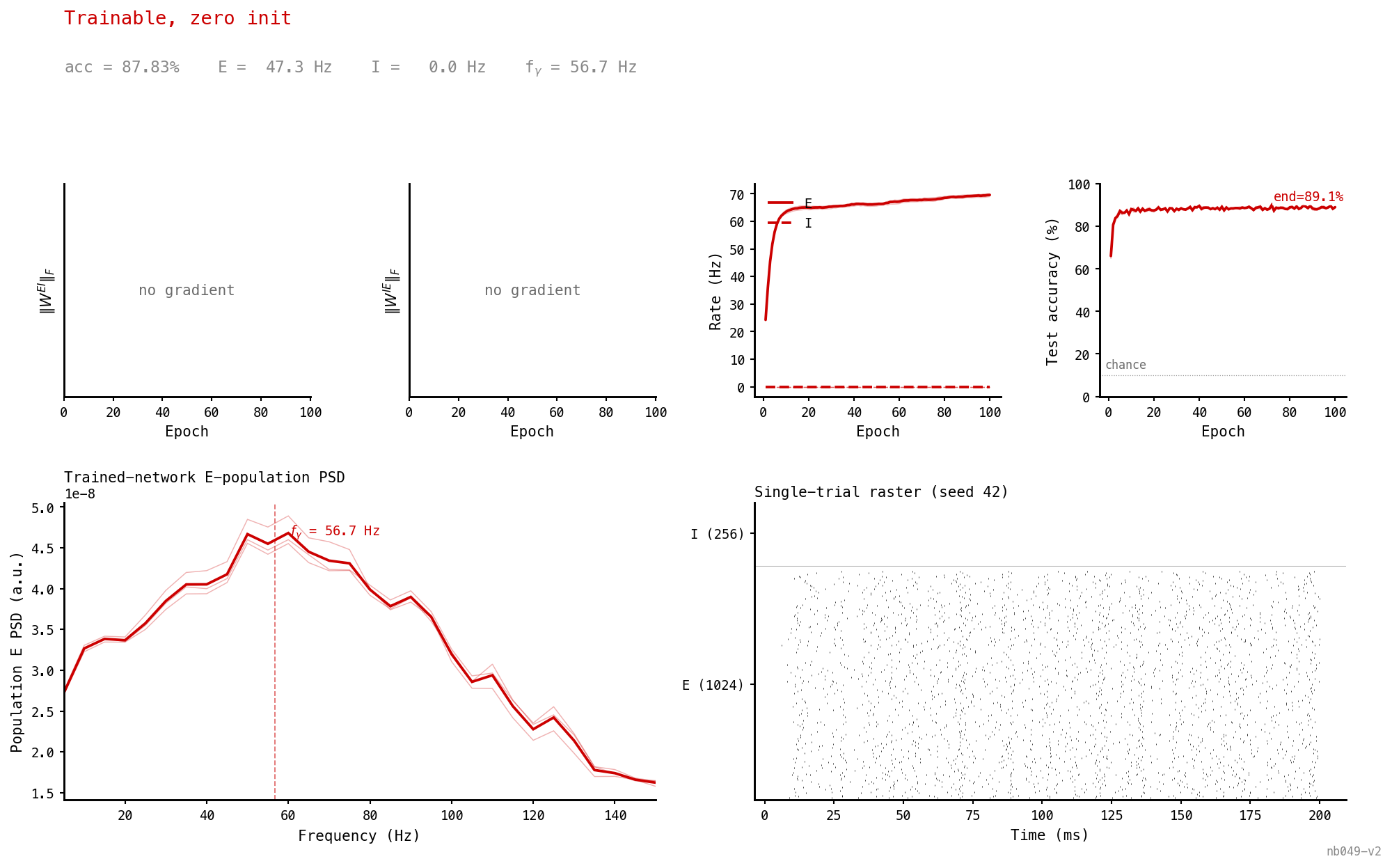
Diagnostic card. Top strip: |W_ei|_F and |W_ie|_F sit at exactly 0 throughout training. E rate climbs from ≈ 5 Hz to ≈ 47 Hz; I rate stays at 0. Accuracy reaches 88% by epoch 25 and plateaus. Bottom-left: PSD peak at ≈ 57 Hz, no low-frequency mass. Bottom-right: single-trial raster shows dense asynchronous E firing; the I row is empty. — Start the loop disabled. Gradient descent never reactivates it: the recurrent weights stay at zero throughout, the network runs as plain COBA, E fires densely, I is silent. Accuracy still 87.8% — within 0.2 pp of the trainable-PING-init case. From a cold start, there’s no gradient path back to PING.

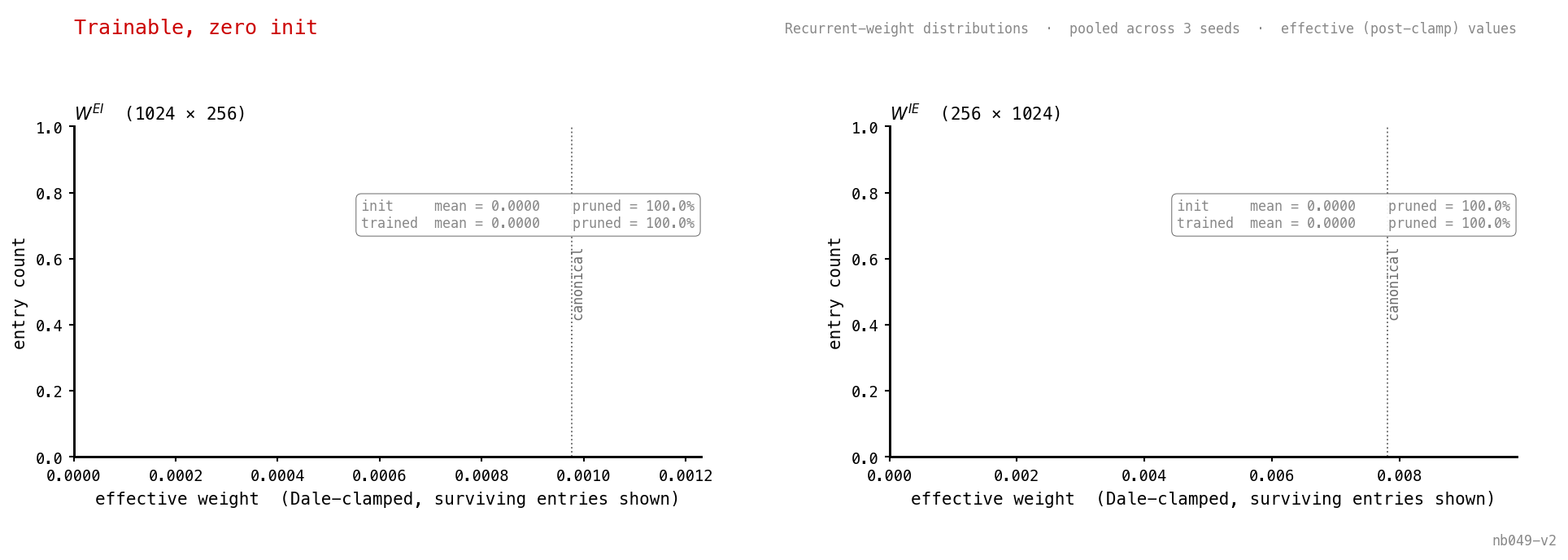
Two-panel histogram. Left: W^EI init and trained both a single spike at exactly zero — 100% pruned. Right: same for W^IE. — Both panels are a single spike at zero. No gradient flows back into a disabled loop, so nothing moves.

Trainable, small initialisation

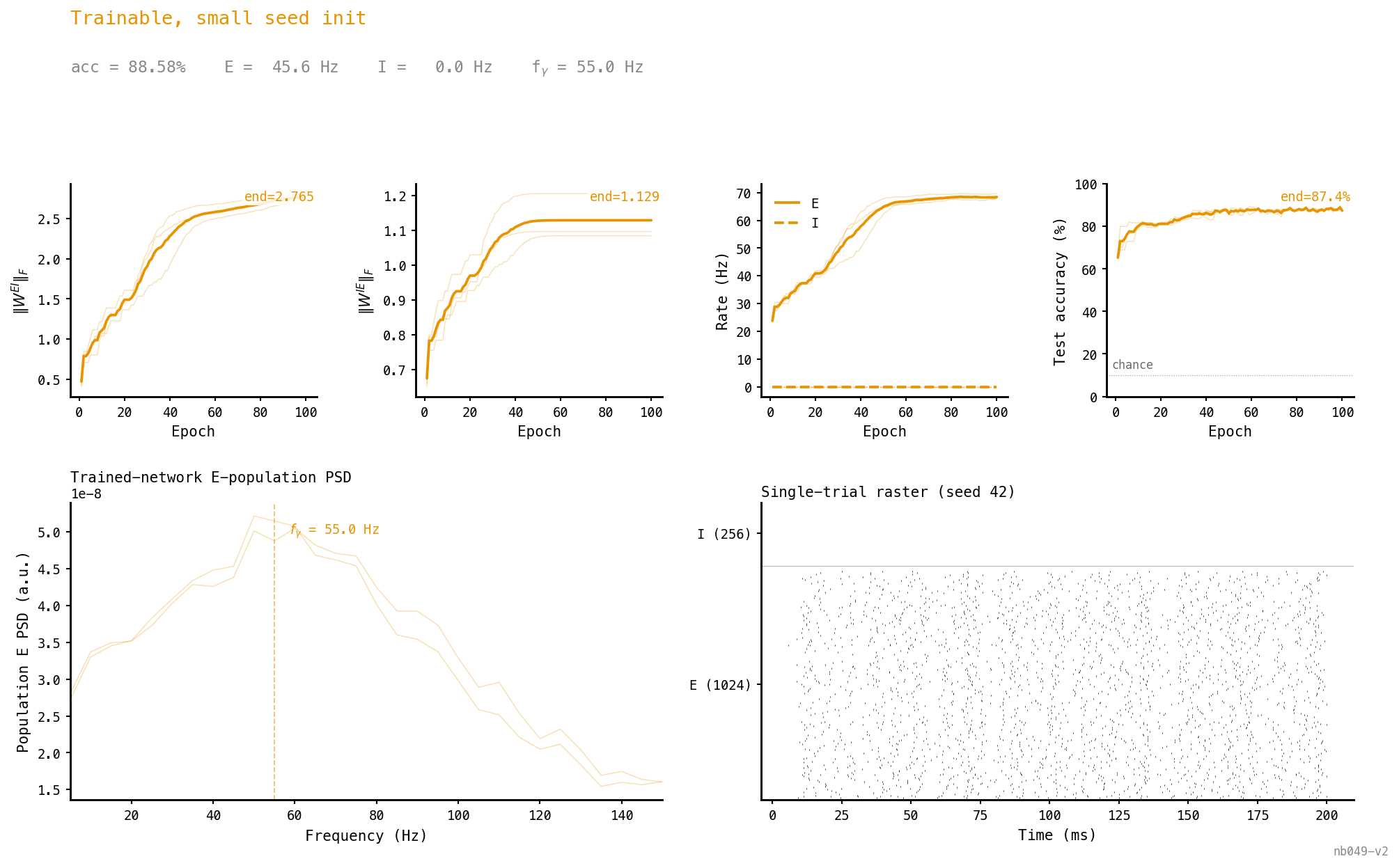
Diagnostic card. Top strip: |W_ei|_F starts at ≈ 0.00010, grows monotonically; |W_ie|_F starts at ≈ 0.00078, grows much less. E rate climbs from ≈ 7 Hz to ≈ 46 Hz; I rate is silenced to 0 within ≈ 15 epochs. Accuracy reaches 88.6% by epoch 25. Bottom-left: PSD peak at ≈ 55 Hz. Bottom-right: single-trial raster shows dense asynchronous E firing; the I row is empty. — Start at 1/10 canonical so there’s a small but non-zero gradient signal in the loop. Same endpoint as the canonical-init case: dense E, silent I, 88.6% accuracy.

Two-panel histogram (effective weight, w<0 clamped to 0, pooled across 3 seeds). Left: W^EI init outline narrow at 0.0001, 0% pruned. Trained fill is a tall spike at 0 (99% pruned) plus a sparse positive tail reaching ≈ 0.005. Effective mean ≈ 0.00002. Right: W^IE init narrow at 0.0008, 0% pruned. Trained fill has a smaller spike at 0 (37% pruned) plus a positive distribution centred near 0.0015. Effective mean ≈ 0.0015. 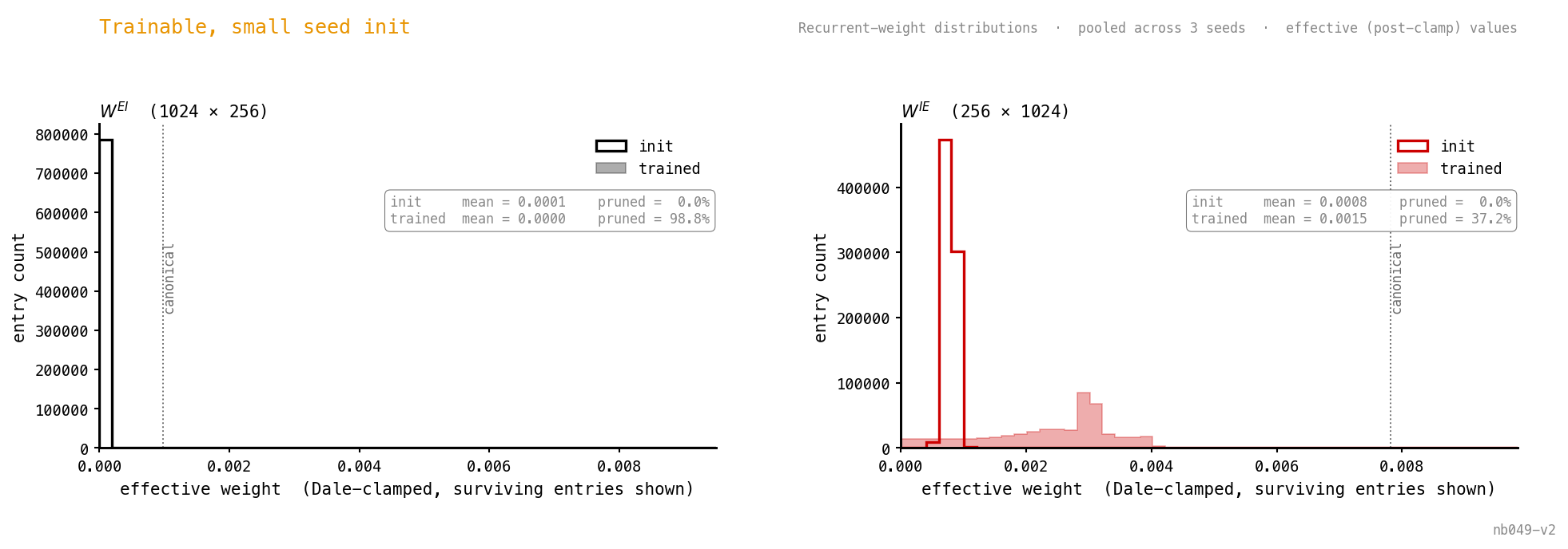— Sharper version of Figure 4: **99% of $W^{EI}$ pruned and 37% of $W^{IE}$ pruned**. The few survivors grow, but the population-level effect is loop dismantling.

At-a-glance comparison (mean across three seeds)

Condition	Acc (%)	$E$ (Hz)	$I$ (Hz)	$f_\gamma$ (Hz)	$W^{EI}$ pruned / eff. mean	$W^{IE}$ pruned / eff. mean
frozen_ping	86.2	8.5	37.9	38	0% / 0.0010	0% / 0.0078
trainable_ping_init	88.0	42.3	0.3	55	73% / 0.0005	0% / 0.0078
trainable_zero_init	87.8	47.3	0	57	100% / 0	100% / 0
trainable_small_init	88.6	45.6	0	55	99% / 0.00002	37% / 0.0015

The frozen control reaches healthy PING; every trainable condition reaches the same dense-E / silent-I attractor at ≈ 88% accuracy — about 2 pp above the control. Starting state doesn’t matter, only whether the loop is allowed to train.

Discussion

The mechanism, in one sentence: Adam drives most $W^{EI}$ entries below zero and Dale’s law clamps them to structural zeros, so the loop loses its drive to I and the gamma shunt that paces E firing disappears.

The naïve view — ” $\lVert W^{EI}\rVert$ grew, so the loop should be stronger” — is what makes the result look paradoxical at first. The Frobenius mean of the absolute stored parameters does grow, because the negative-stored pruned entries contribute their absolute values to that average. But that’s not what the network sees: the forward pass clamps them, the effective mean drops below init, and the dynamics behave as if the matrix has been sparsified to ≈ 16% of its connectivity with a strong-but-rare survivor pattern. The few I cells still receiving drive can’t gate the whole E population.

This makes the rate-floor framing in ar009 / ar010 more honest about its scope. The mechanism $r_E = p \cdot f_\gamma$ requires the gamma cycle, which requires the loop to remain biophysically scaled. MNIST does not select for that — if anything it selects against it, since the dense-fire COBA attractor scores 2 pp higher. The argument is therefore “freezing the loop gives a rate-bounded sparse code that streams cleanly”, not “the network would find this regime on its own”. Whether a streaming or continuous-input task changes the calculus — by making the readout pay for dense-fire saturation — is the natural follow-up, started by nb048.

Two caveats:

Two cells NaN’d late in training (trainable_ping_init seed 42, trainable_small_init seed 44). Their pre-NaN trajectories matched the surviving seeds; final-state numbers average the non-NaN cells. The collapse story doesn’t depend on them.
MNIST is thin. One-shot 200-ms classification with a permissive linear readout doesn’t reward temporal sparseness. A task that does is the cleanest follow-up.

Next steps

Streaming task with trainable loop. Run this experiment on the streaming-MNIST protocol from nb048 — does the dense-fire attractor still win when the readout is sensitive to over-saturation?
2D init sweep. Sample $(W^{EI}, W^{IE})$ initial means across a plane and map the attractor basins.
$\tau_\text{GABA} \times$ trainability. Does changing the I time constant shift which attractor wins?
Anti-pruning regulariser. Penalise either $|W^{EI} -$ canonical $|$ or low gamma-band PSD and ask how strong the penalty has to be before Adam stops dismantling the loop.