023 — PING fundamentals

Abstract

Strips PING down to its biophysical fundamentals and characterises it in isolation from any task — no training, no readout, no loss, just a free-running network driven by Poisson input. The E → I → E loop produces gamma at ≈30 Hz with the standard $\tau_\text{AMPA} + \tau_\text{GABA}$ cycle period, and the f-I curves show the loop is dynamic-range compression: PING holds E an order of magnitude below COBA across two orders of magnitude of drive, while COBA saturates near its refractory ceiling.

Methods

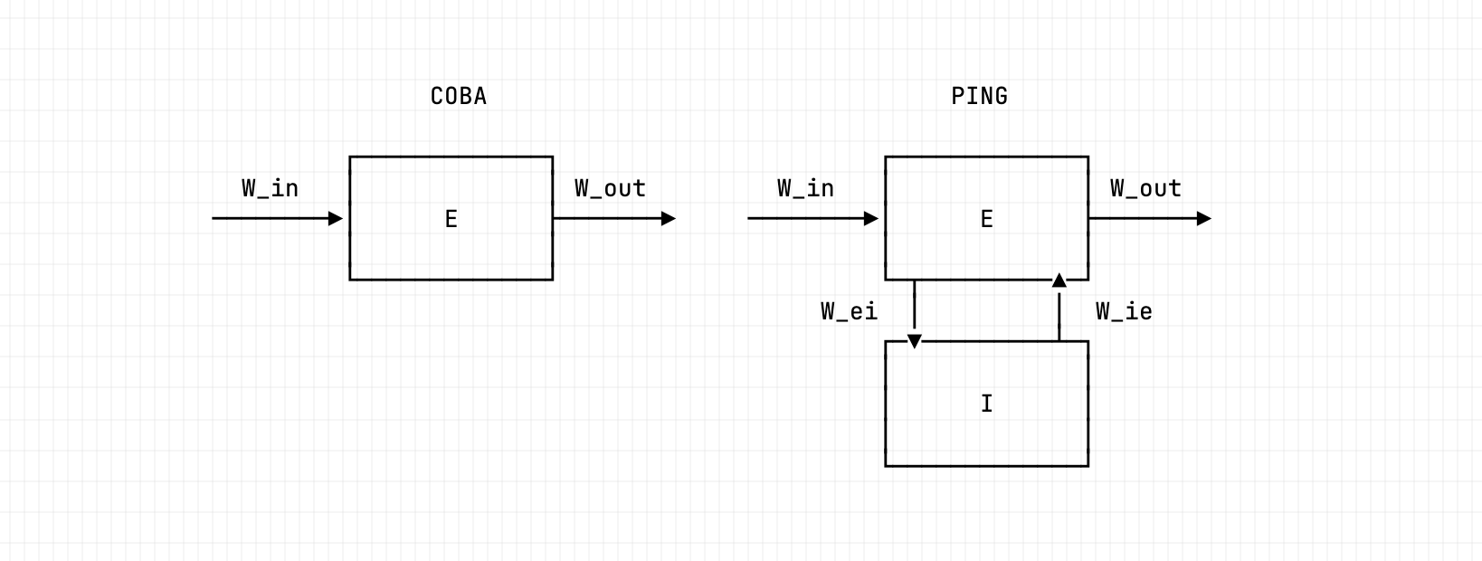
Schematic of the PING network: an input layer projects through W_in to the excitatory (E) population; E projects to the inhibitory (I) population through W_ei, and I projects back to E through W_ie, forming the recurrent E→I→E loop. There is no I→I synapse. — The PING architecture characterised in this notebook. An input layer drives the excitatory population through $W_\text{in}$ ; the E→I→E loop is formed by $W_\text{ei}$ (E to I) and $W_\text{ie}$ (I back to E), with no I→I synapse. Disabling the I→E loop (*ei-strength 0*) recovers the COBA reference; engaging it (*ei-strength 1.5*) produces the gamma rhythm.

The full conductance-based model that produces PING is documented in COBANet; this notebook is the empirical companion piece. Two conditions are run on the same network: ei-strength 0 (loop disabled, the COBA reference) and ei-strength 1.5 (loop engaged, the PING regime). MNIST digit 0 drives the input layer through trained $W_\text{in}$ . The rate sweep at the end replays the trained PING baseline from nb025 (seed 42, $\theta_u =$ off) over a sweep of input rates, with both MNIST and spatially uniform Poisson drive.

Results

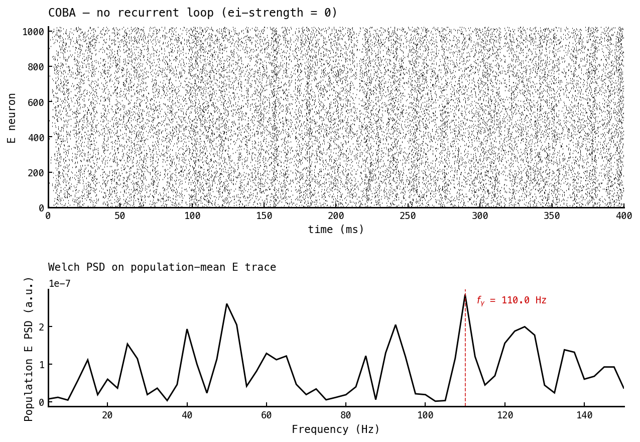
Two-panel figure. Top: E spike raster across 400 ms, asynchronous firing across the population, no I-population activity (loop disabled). Bottom: Welch PSD on the population-mean E spike trace over 5–150 Hz. No isolated gamma peak — the spectrum has scattered weak peaks driven by the feedforward input structure, not by a recurrent cycle. — Baseline: recurrent inhibitory loop silent (*—ei-strength 0*). The E raster fires asynchronously across the full 400 ms; the I population is silent. The Welch PSD on the population-mean E trace (computed exactly like nb041 and nb049: one window per trial, `nperseg = T`, parabolic-interpolated peak) shows **no isolated gamma peak** — only the broadband structure of input-driven asynchronous firing. This is the “PING off” reference for the next figure.

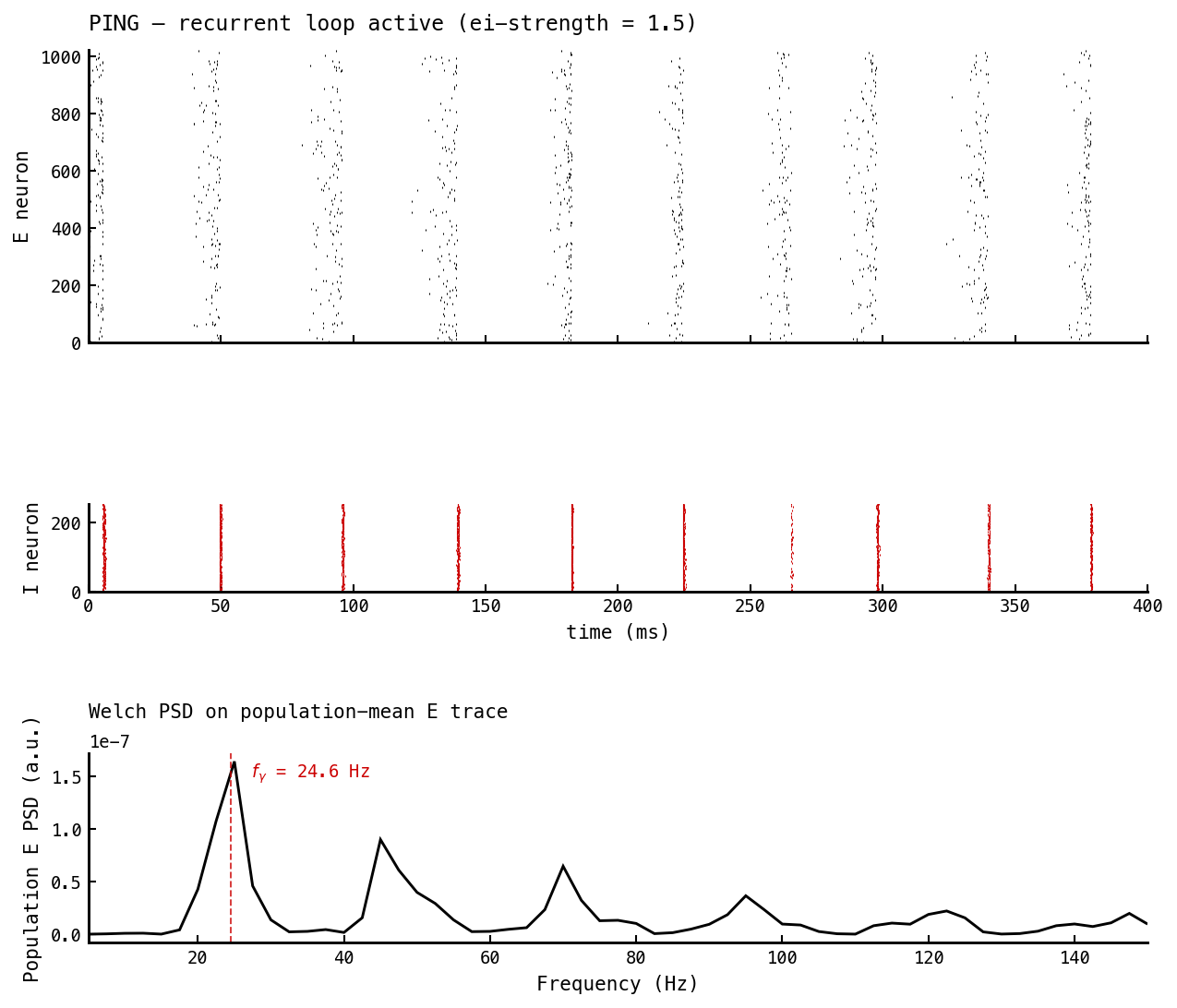
Three-panel figure. Top: E spike raster across 400 ms showing vertical bands every ~45 ms. Middle: I spike raster showing synchronous bursts trailing each E-burst. Bottom: Welch PSD on the population-mean E trace, sharp gamma peak at f_γ ≈ 24 Hz marked with a dashed vertical line, with harmonics at ≈ 48, 72, 96, and 120 Hz. — Same network with the I→E loop turned on (*—ei-strength 1.5*). Same MNIST input, same integration window. The E raster now shows vertical bands and the I population fires synchronous bursts trailing each E-burst by the AMPA delay. The Welch PSD has a **clean gamma peak at $f_\gamma \approx 24$ Hz**, with the periodic burst structure visible as harmonics at the higher integer multiples — the spectral signature of the recurrent E↔I loop that the COBA panel lacked.

COBA single-neuron traces. Three panels for the most active E neuron — voltage, conductances, signed currents — with no I-loop activity to show.

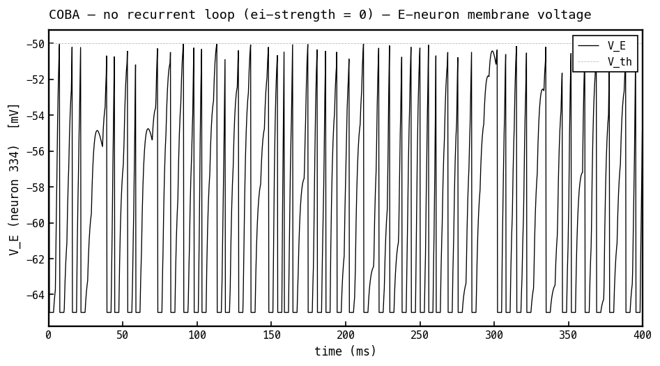
V_E (black) for one E neuron over 400 ms with the recurrent loop off (COBA). V_E charges toward threshold V_th = −50 mV (faint dashed) and hard-resets to V_reset = −65 mV at each spike, with no rhythmic envelope. — Membrane voltage $V_E$ (black) of the most active E cell over 400 ms with the recurrent loop **off** (COBA mode, *ei-strength 0*). Driven only by feedforward input, the cell just charges toward threshold ( $V_\text{th} = -50$ mV, faint dashed) and hard-resets to $V_\text{reset} = -65$ mV each time it fires — irregular, input-paced spiking with no rhythmic structure. This is the rhythm-free control for the PING version in Figure 4a, where inhibition carves a gamma envelope into the same trace.

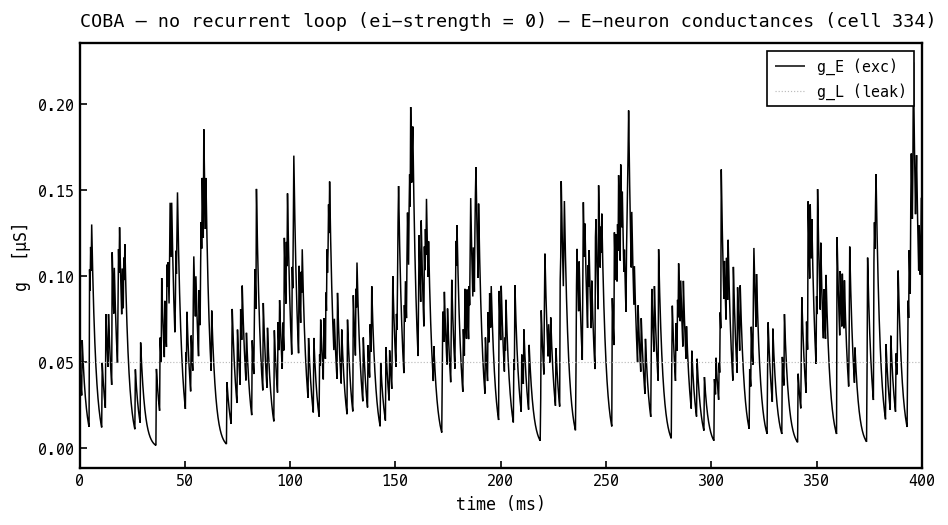
Conductances on the E neuron in COBA mode: g_E (black) and g_L (faint dotted), both non-negative. No g_I trace because the I→E loop is disabled. — Synaptic and leak conductances on the same E cell, COBA mode. Only the excitatory conductance $g_E$ (black) is active — it steps up with each arriving input spike and decays with $\tau_\text{AMPA}$ — while the leak $g_L$ (faint dotted) is a fixed constant. There is no inhibitory $g_I$ because the I→E loop is off. All conductances are **non-negative**: they count open channels, not current direction or sign.

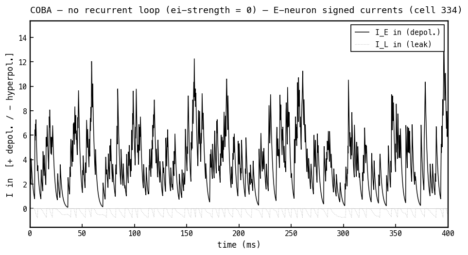
Signed currents into the E neuron in COBA mode: I_E in (black, positive = depolarising), I_L (faint dotted, near zero). No I_I trace because the loop is off. — Signed synaptic currents into the E cell, COBA mode, with $I_X^\text{in} = -g_X (V - E_X)$ (positive = depolarising, i.e. pushes $V$ up). With no inhibition, the only synaptic current is the depolarising excitatory current $I_E^\text{in}$ (black); the leak current (faint) hovers near zero. Compare Figure 4c, where adding the loop introduces an inhibitory current of the *opposite* sign.

PING single-neuron traces. Six panels: three for the most active E neuron, three for the most active I neuron. The E panels are where the “sign lives in the driving force” picture becomes literal.

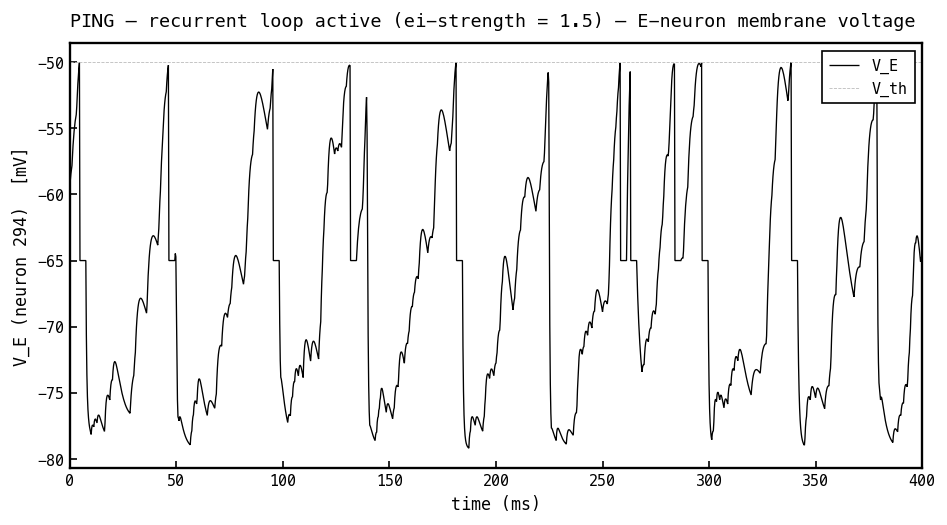
V_E (black) for one E neuron with the recurrent loop on (PING). Rhythmic inhibitory bursts hold V_E below threshold, dragging it toward −80 mV each cycle; it recovers and may fire only as g_i decays between bursts. — Membrane voltage $V_E$ (black) of the most active E cell with the recurrent loop on (PING mode, *ei-strength 1.5*), same input as the COBA panel 3a. Now the rhythmic inhibitory bursts hold the cell below threshold most of the time: each I-burst drags $V_E$ down toward $E_i = -80$ mV, and the membrane recovers — and can fire — only as the inhibition decays between bursts. The gamma rhythm is visible directly in the voltage; the loop has turned the irregular firing of 3a into cycle-gated firing.

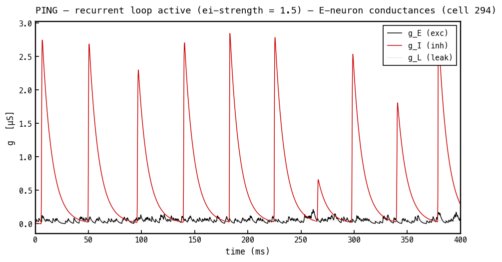
Conductances on the E neuron in PING mode: g_I (red) in large rhythmic bursts, g_E (black, small), g_L (faint dotted). All non-negative; g_I dominates and oscillates at the gamma cadence. — Conductances on the same E cell, PING mode. The inhibitory conductance $g_I$ (red) now dominates — it spikes once per gamma cycle as the synchronous I-burst arrives through $W_\text{ie}$ , then decays with $\tau_\text{GABA}$ — while the excitatory $g_E$ (black) carries the smaller feedforward input and $g_L$ (faint) is fixed. All three traces are **non-negative**: $g_I$ is large and positive, and that is what shunts the cell — it carries no sign of its own.

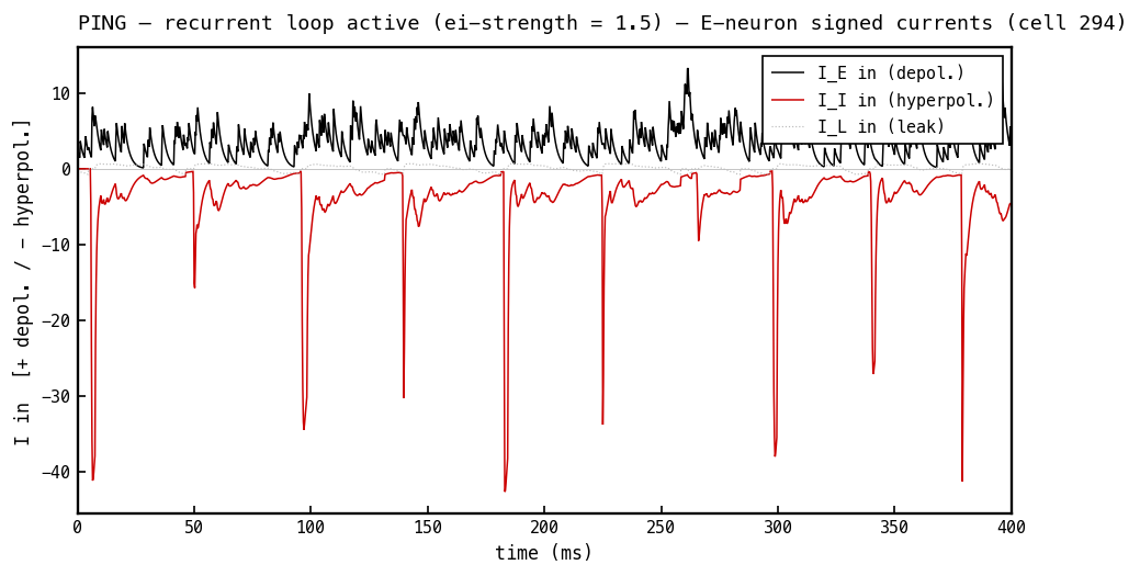
Signed currents into the E neuron in PING mode: I_E in (black, positive = depolarising), I_I in (red, negative = hyperpolarising) with sharp downward pulses at each I-burst, I_L (faint dotted, near zero). I_I is negative even though g_I is positive — the sign is from (V − E_i) > 0. — The load-bearing panel. Signed currents into the E cell, PING mode. The excitatory current $I_E^\text{in} = -g_E(V - E_E)$ (black) is positive (depolarising). The inhibitory current $I_I^\text{in} = -g_I(V - E_I)$ (red) is **negative (hyperpolarising) even though $g_I$ is positive** (Figure 4b) — the minus sign comes entirely from the driving force $(V - E_I) > 0$ whenever $V$ sits above $E_i = -80$ mV. This is the COBA principle made literal: *the sign lives in the driving force, never in the conductance.* The sharp negative pulses are the per-cycle inhibitory kicks that gate the rhythm.

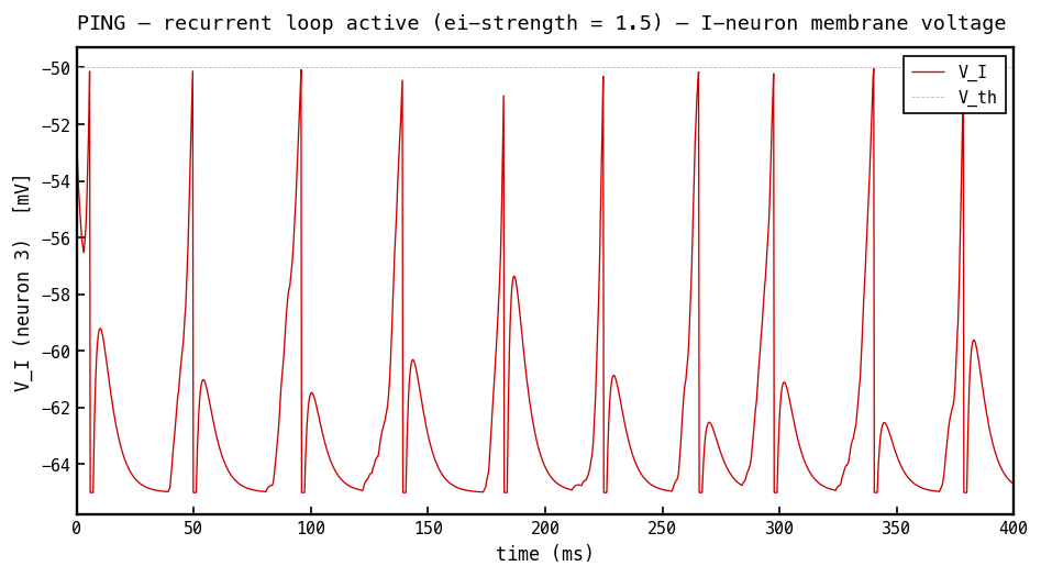
V_I (red) for one I neuron in PING mode. V_I ramps up with the E-burst volley, crosses threshold V_th = −50 mV, resets, and fires once per gamma cycle. — Membrane voltage $V_I$ (red) of the most active I cell, PING mode. The I cell integrates the excitatory volley from the E population and fires once per gamma cycle, so $V_I$ tracks the E-burst envelope — ramping up as E cells fire, crossing threshold ( $V_\text{th} = -50$ mV, faint dashed), resetting, and waiting for the next volley. This single I-spike per cycle is what delivers the inhibitory burst seen on the E cell in 4b–4c.

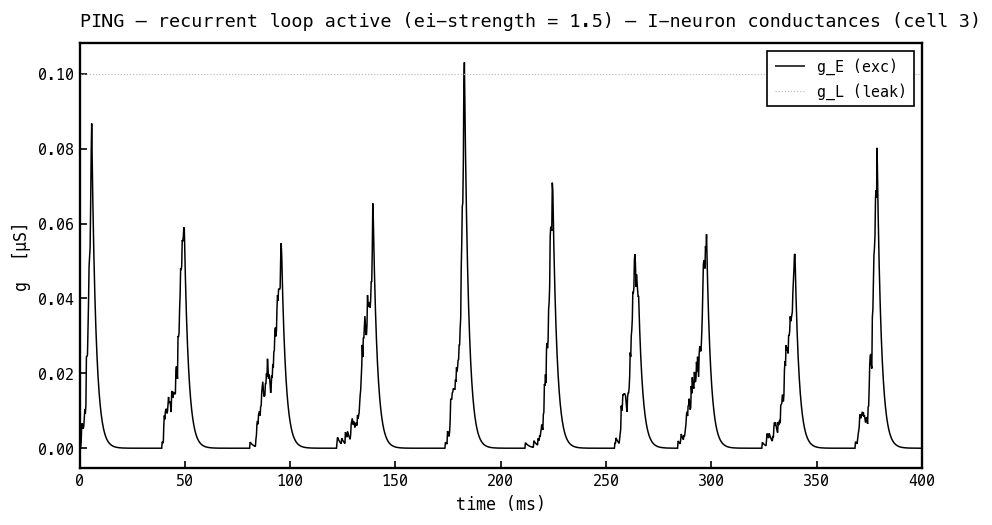
Conductances on the I neuron: g_E (black) tracking the E-spike envelope, g_L (faint dotted) fixed. No g_I because the I neuron receives no inhibition. — Conductances on the I cell, PING mode. The I cell receives **only excitation**: $g_E$ (black) is the arriving E-spike envelope (delivered via $W_\text{ei}$ ) and $g_L$ (faint) is the fixed leak. There is no inhibitory conductance — the architecture has no I→I synapse — which is exactly why the I population can synchronise into the sharp once-per-cycle bursts that clock the loop.

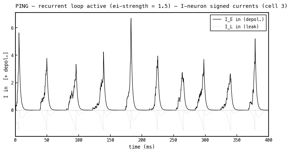
Signed currents into the I neuron in PING mode: only I_E in (black, positive = depolarising) and a small leak current. No I_I trace because the I neuron receives no inhibition. — Signed currents into the I cell, PING mode. With no inhibitory input, only the depolarising excitatory current $I_E^\text{in}$ (black) and a small leak current contribute — the I cell is driven purely up to threshold. Read 4a–4f together and the loop is in cross-section: E spikes ramp $g_E$ on I (4e–4f) → I fires once per cycle (4d) → that spike delivers the inhibitory burst $g_I$ on E (4b) → its negative current shuts E down (4c, 4a) → $g_I$ decays → E refires. That delayed E→I→E loop is PING.

Input-rate sweep

The rasters and traces above are at a single working point. Sweeping the Poisson input rate across the trained PING baseline (nb025, seed 42, $\theta_u =$ off) shows how the network responds to drive: silent below a recruitment threshold, gamma-locked above it, with cycle period invariant to further drive once the loop engages.

Ten stacked raster panels showing trained PING on MNIST digit 0 at input rates from 0 to about 23 Hz; E spikes in black, I spikes in red. Each panel is labelled with the input rate, the per-cell E rate, and the per-cell I rate. At low input (0–5 Hz) the network is silent (E and I rates both 0). At ≈8 Hz input the I-loop engages (I rate jumps from 0 to ≈10 Hz). Above engagement the E rate saturates near 4–5 Hz while the I rate climbs from ≈10 to ≈25 Hz. 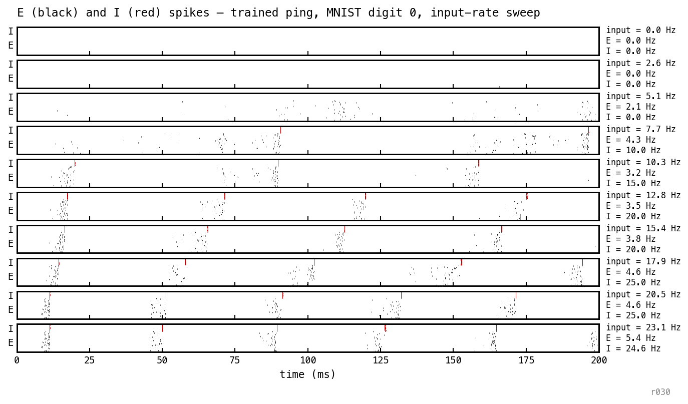— Trained PING (the nb025 baseline) replayed on MNIST digit 0 across ten input-rate values from 0 up to ≈ 23 Hz; each panel is one rate, E spikes (black) above I spikes (red), labelled with the input rate and the resulting per-cell E and I rates. Reading down the stack: at low drive the network is **silent** (E and I both 0); past a recruitment threshold (≈ 8 Hz input) the **I-loop catches** — the I rate jumps from 0 to ≈ 10 Hz and gamma bands appear in the E raster; above that the **E rate stays pinned near 4–5 Hz** while the I rate keeps climbing toward ≈ 25 Hz, and the cycle period barely moves with further drive. (The faint clustering in the just-engaged panels, where I is still 0, is feedforward input structure rather than PING — see the note below.)

At rate = 0 the network is silent. Above a recruitment threshold a few E units fire, the I loop catches, and the gamma cadence appears. Once the loop is locked the cycle period is invariant to further increases in input rate.

A subtlety in the just-engaged panels (e.g. input $\approx 5$ Hz, E = 1.7 Hz, I = 0): the E spikes look mildly clustered even though the I-loop hasn’t fired. This is feedforward — not PING. The Poisson input stream has natural temporal fluctuations, the digit-0 input is spatially correlated, and the trained $W_\text{in}$ has learned to be selective for digit-relevant pixels. So the cells that fire are the input-tuned subset, and they fire together during input-rich windows. The participation pattern is partially preserved from training; the gamma timing is not, because the loop is genuinely off.

To isolate the bare drive-response of each architecture, repeat the sweep with a spatially uniform input — every input channel firing at the same Poisson rate, with no digit structure — and compare PING against COBA on the same axes.

Two-panel figure, both panels on the same y-axis (0 to ≈ 320 Hz). Left (COBA, no I-loop): E rate (black, circles) climbs steeply and saturates toward ≈ 310 Hz at 100 Hz input; I rate (red) flat at zero. Right (PING, I-loop active): E rate (black) held low, reaching only ≈ 30 Hz at 100 Hz input, while I rate (red, squares) and the E+I total (amber dashed) climb to ≈ 155 and ≈ 185 Hz — far below COBA's E. On the shared scale the PING curves sit in the lower fifth of the axis. 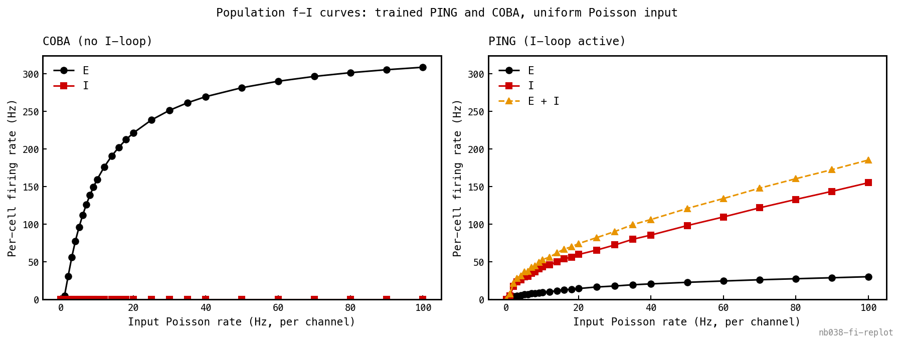— Population f-I curves — mean per-cell firing rate vs input Poisson rate — for trained COBA (left) and trained PING (right) under spatially **uniform** input (all 784 channels at the same rate, no digit structure), **both panels on a shared y-axis** so the compression is read on one scale. **COBA** (left): E (black) climbs steeply and saturates toward its refractory ceiling (≈ 310 Hz at 100 Hz input — every cell firing about as fast as it can), with I (red) flat at zero because the loop is disabled. **PING** (right): a recruitment cliff at low input where the I-loop engages, after which E is held ≈ 10× lower than COBA across the range — only ≈ 30 Hz at 100 Hz input where COBA runs to ≈ 310. The I curve (red) and the E+I total (amber) ride *above* the E curve: I fires harder than E to suppress it. This is the *function* of PING — **dynamic-range compression**, folding drive that would saturate E into a bounded gamma cadence.

Two qualitative responses to the same drive, on one shared y-axis. COBA (left) rises sharply across 1–10 Hz input then saturates toward its refractory ceiling ( $\approx 310$ Hz at 100 Hz input — every E cell firing essentially as fast as it can); the I rate stays at zero because the loop is off. PING (right) shows the recruitment cliff at low input and then holds E roughly an order of magnitude lower than COBA across the entire post-engagement range — $\approx 30$ Hz at 100 Hz input against COBA’s $\approx 310$ . The I curve sitting above the E curve at every input rate is the visual signature of the loop — I has to fire harder than E to suppress it. The I-loop is doing dynamic-range compression — pulling drive that would saturate the E population into a bounded gamma cadence.

Discussion

The signed-current picture (Figure 4c) is the load-bearing observation: $g_I$ stays non-negative throughout, but the current it drives is negative because $(V - E_I) > 0$ — sign lives in the driving force, never in the conductance. The f-I curves make the function of the loop visible: PING is dynamic-range compression, not just rhythm. E rate stays an order of magnitude below COBA across two orders of magnitude of input, while COBA saturates near its refractory ceiling.

Next steps

Sweep $\tau_\text{AMPA}$ and $\tau_\text{GABA}$ independently and confirm the gamma peak tracks $1/(\tau_\text{GABA} + \tau_\text{AMPA})$ .
Repeat the f-I curves with a sweep of refractory period and check whether COBA’s saturation point lines up with the predicted $1/\tau_\text{ref}$ ceiling.