047 — Per-event shunt magnitude sets rates, not summed inhibition
Abstract
How many inhibitory cells does a PING network need? We sweep from 0% to 25% of the excitatory pool ( fixed) on an untrained network and ask how the per-cell firing rates respond. The answer depends on how you scale the synapses with : under constant per-edge weights — the biologically motivated choice — rates are flat across the sweep, even when the summed inhibitory drive varies by ≈ 250×. Under synaptic () or critical-balance () scaling the rates reduce slightly at small . What the network cares about is the per-event shunt magnitude, not the time-averaged total drive — and only constant-per-edge holds that fixed.
Methods
Simulation. Untrained PING net at ms, fixed, swept over 256 (the 25% points, with 0% implemented as ). Reference per-edge weights μS and μS at the canonical . Drive: uniform 25 Hz Poisson input on 784 channels, ms, 4 trials per cell. Reported rates are per-cell averages over trials; rasters come from trial 0.
Three scaling regimes. When we change we have to decide what happens to the strength of each individual synapse. There’s no neutral choice — the three standard conventions disagree even on what “the same network at different sizes” means. All three coincide at the canonical anchor and only differ once we shrink .
The intuition: the network is all-to-all between layers, so each E cell receives one I→E synapse per I cell — i.e. incoming I→E synapses per E cell, with a per-edge weight on each. When we change we have to decide what happens to that per-edge weight. We can keep it fixed (so total drive into each E cell grows with the pool), rescale it as (so total drive stays put), or split the difference. These correspond to:
-
Constant per-edge — the per-edge weight is fixed at no matter how big or small the I pool is. Each I→E connection that exists has the same strength as it would in the canonical 256-cell network. Drop from to and an E cell now has one incoming I→E synapse where it used to have 256 — total inhibitory conductance into each E cell drops by .
-
Synaptic normalization () — per-edge weight scales as , so the time-averaged total drive into each E cell is held fixed by construction: more I cells but weaker individual synapses, or fewer I cells but proportionally stronger synapses. At the lone I→E connection is stronger per edge to compensate for the missing 255 contributions. This is the classic mean-field convention: it says “what the cell receives on average” is the meaningful quantity, and population size is just a knob for sampling resolution.
-
Critical balance () — per-edge weight scales as , the geometric mean of the other two. Brunel and collaborators argued in the asynchronous-irregular literature that this is the “right” scaling for a balanced-state network: it keeps the variance of summed input invariant while letting the mean grow as , which is what you’d want if E firing is driven by input fluctuations around the inhibitory floor rather than by deterministic threshold crossings. At each I→E edge is stronger than reference; at it’s unchanged.
The three regimes thus encode three different stories about what the network is “really” doing — fixed-anatomy, mean-balanced, or variance-balanced. Running all three on the same sweep is the cleanest way to ask which story actually fits the dynamics.
Results
Constant per-edge
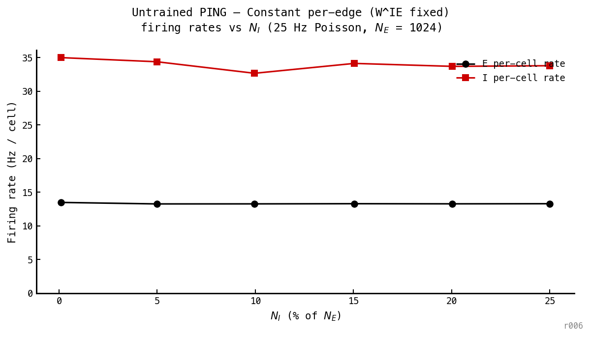
E and I per-cell rates are invariant to across the 0–25% sweep — Hz and Hz everywhere. The 0% point (one I cell) lands within 1% of the canonical 25% point (256 I cells).

The gamma cycle (≈ 28 ms cadence) is identical across the sweep. The I row gets denser as grows; the E burst pattern is unchanged.
Synaptic normalization ()
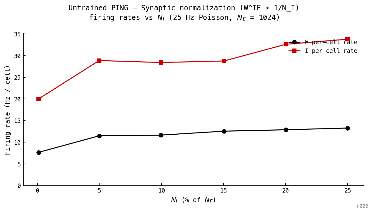
Rates drop at small — opposite of the naïve mean-field prediction. At , falls to 7.7 Hz (vs 13.5 Hz under constant per-edge). All three regimes converge at .
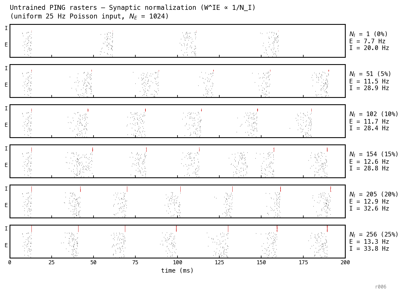
At the lone I cell carries a μS synapse to each E cell. One I spike clamps the E population for many ms — the cycle stretches and E firing thins.
Critical balance ()
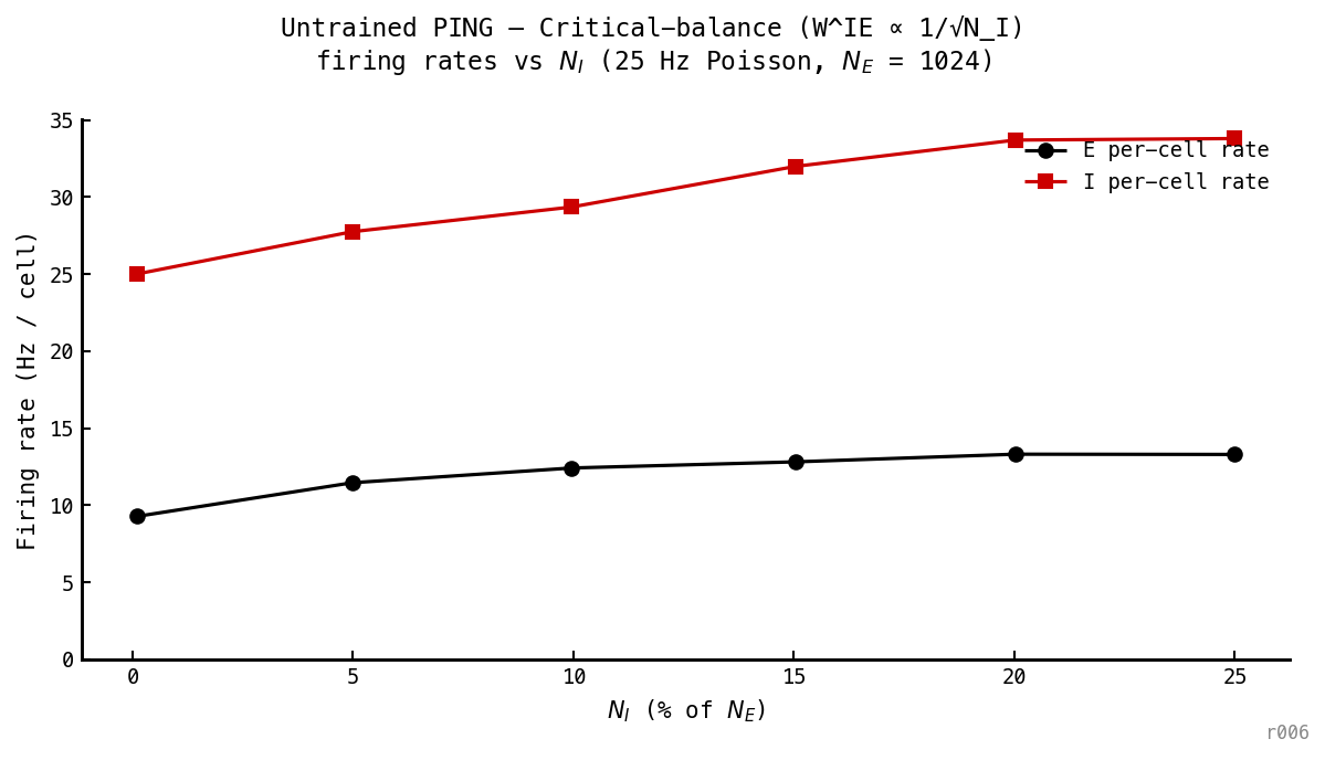
Intermediate between the other two regimes: at , Hz. Even a per-event scaling is enough to perturb the cycle dynamics.
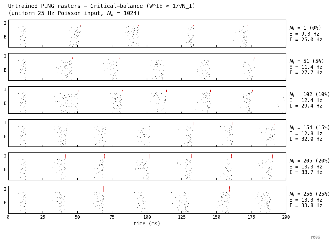
At the per-edge is — between synaptic norm’s and constant’s . Cycle distortion scales accordingly.
Discussion
Why is constant per-edge flat? Three things have to hold simultaneously for the rates not to move with :
- Summed inhibition is the wrong quantity. It grows ∝ (≈ 250× across the sweep) and yet doesn’t budge — so the loop is not in a regime where time-averaged total drive sets the rate.
- Per-I-cell drive is fixed. Each I cell still receives the same E → I input regardless of , so is set by single-cell biophysics, not by population size.
- Cycle frequency is fixed. The gamma clock period depends on , , and loop gain (nb033). is independent of at fixed per-edge weights, so the per-cycle Bernoulli participation gate sets at a pool-size-invariant rate.
The synaptic and critical-balance regimes are the falsifier. Synaptic normalization holds the time-averaged mean drive exactly constant — and rates still drop at small . The thing the network actually responds to is the per-event shunt magnitude: one huge shunt and many small ones aren’t the same, even when their time-averaged drive is identical. Only constant per-edge keeps the per-event magnitude fixed across the sweep.
This matches nb046’s structural-bound reading: rate is set within each cycle (does the cell cross threshold before the next I-shunt?), not by mean-field balance across cycles.
Two caveats:
- Untrained network. After training, adapts and the per-cell operating point shifts; whether the -invariance survives training is a separate question.
- 0% endpoint approximation. stands in for 0%. Literal would disable the I-loop entirely and collapse to COBA — see nb025 Figure 1.
Next steps
- After-training check — does the -invariance survive training, or does the readout pick a preferred that depends on pool size?
- map — locate the recruitment cliff in two dimensions.
- map — test whether the affine slope in is -invariant.
- Direct per-event measurement — measure the post-I-burst E-firing-suppression window under each regime and check it correlates with the rate drop.